Qubit characterization

In previous courses we always studied closed systems, in which the evolution of the quantum state is deterministic, which is to say that given an Hamiltonian we can predict the evolution of the system (qubit) in the future. In the real world (open system) things are different because our system (qubit) interacts with uncontrolled degrees of freedom like the environment and various noise sources.

Noise

We can classify noise into two categories: systematic noise and stochastic noise.

Systematic noise

Systematic noise is the one that arises from poor management of the experiment or readout errors. For example if we apply a microwave pulse to the qubit that we believe will impart a 180 rotation and the control field is not tuned properly we might get a different angle of rotation (e.g. 183).

The nice thing about this kind of noise is that it is systematic, which means that it can be corrected by proper calibration.

Stochastic noise

Stochastic noise, on the other hand, arises from random fluctuations of parameters that are coupled to the qubit, such as the thermal noise of a resistor in the control line, external magnetic fields, etc.

These unknown and uncontrolled fluctuations lead to decoherence.

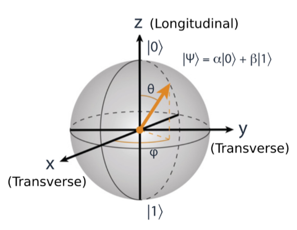
Bloch sphere representation

todo

Density matrix

From what we saw in the introduction the density matrix can be expressed as and can be expressed in terms of and or in terms of Pauli matrices :

where is the Bloch vector.

If is a unit vector we are in a pure state, otherwise if we will have a mixed state.

The problem with this form of the density matrix is that it doesn’t take into account the effect of noise on the qubit.

In the following we will see a model that solves this issue but before doing this we need to study how decoherence affects the qubit.

Decoherence in transmon qubit

Decoherence in a qubit refers to the process by which the quantum coherence of the qubit is lost due to interactions with its surrounding environment.

Decoherence can be categorized into:

• Longitudinal relaxation
• Pure dephasing
• Transverse relaxation

Longitudinal relaxation

The longitudinal relaxation describes depolarization along the qubit longitudinal axis (z-axis). it is often referred to as energy decay or energy relaxation because it makes the excited qubit return to the ground state (which, in superconductive qubits is the steady state).

For a complete description of the relaxation we have to consider that there are two components that play a role in the transition of the state:

• is the up transition and makes the qubit go from to , i.e. from the ground state to the excited state.
• is the down transition and makes the qubit go from to , i.e. from the excited state to the ground state.

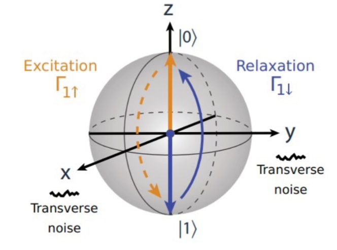
The longitudinal relaxation rate is defined as follows:

has an exponential decay and represents the time that the qubit takes to reach the steady state value.

Even though the decay rate is the sum of two contributions, the up transition (the one that excites the qubit) is negligible. For example of a qubit that operates at and we would have

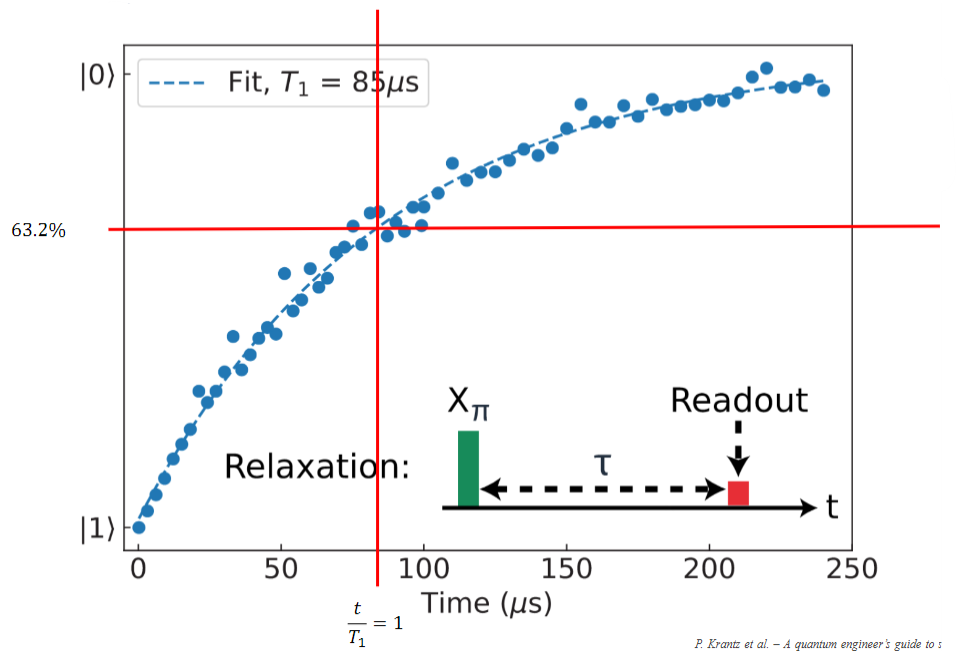
Longitudinal relaxation measurement

To be able to measure the value of we can perform a series of measures that will give a series of points that will exponentially tend to the ground state. The procedure is as follows:

1. Prepare the qubit in the excited state using -pulse (we could also use )
2. Wait for a time
3. Measure the qubit, this operation will project the state into either or
4. Repeat the steps above several times with the same and average the results to get a single point
5. Repeat all the steps above changing each time to obtain a series of points
6. Fit the points with a curve proportional to

At we have a decay of the exponential.

P. Krantz et al. – A quantum engineer’s guide to superconducting qubits, Appl. Phys. Rev. 6 (2019)

Dephasing

Traverse relaxation (decoherence)

Bloch-Redfield model

Qubit control