2DEG

2D Electron Gas

Now we will study the case in which we have an almost intrinsic material in an heterostructure with an heavily doped one. In this case electron start to diffuse form the left-hand side (the heavily doped material) to the right-hand side, this effect is called remote doping or modulation doping.

n: almost intrinsic N: heavily doped

So some electron flow from the left-hand side (the heavily doped material) to the right-hand side, as it has a lower energy conduction band. Doing that they loose energy and become trapped because they cannot climb the barrier formed by the band bending. Furthermore the discontinuity in the band prevents the electric filed to return the electrons to the donors, and contribute at squeezing the electrons on the triangular potential well just formed.

The green line in the drawing is the tangent to the conduction band which can be used as an approximation for a triangular potential well, the width of the well is typically around 10 nm.

For sufficiently thin potential wells and moderate temperatures, only the lowest energy level (typically the ground state) is occupied. Consequently, the motion of electrons in the direction perpendicular to the interface (z direction) can be disregarded. However, electrons retain freedom to move parallel to the interface, making it quasi-two-dimensional. Within the well, the planar motion of electrons experiences weak scattering due to the absence of dopants (specifically ionized impurity scattering) (the well is located in the “n” region). Modulation doping proves to be an effective strategy for reducing donor electron scattering. This reduction in scattering is crucial for enhancing mobility.

Inside the two-dimensional electron gas (2DEG), the mobility is remarkably high. Hence, this structural arrangement is well-suited for constructing high-speed devices such as High Electron Mobility Transistors (HEMTs).

Electronic levels for 2DEG

We can consider the 2DEG an area where the electrons are free to move in the (,) direction and confined by a triangular well in the direction.

We can assume that and are macroscopic quantities and that . Applying the Free electron model, considering the potential constant and equal to zero in the (,) direction and we can write the Schrödinger equation:

since the potential depends only on we can look for solution like:

substituting in the SE we get:

we can split into two terms and get

Equation describes free electrons in the plane (where the potential is constant) and thus we get plane waves:

Note

Notice that should be the effective mass in the real calculation

Applying the PBC to the and directions we get

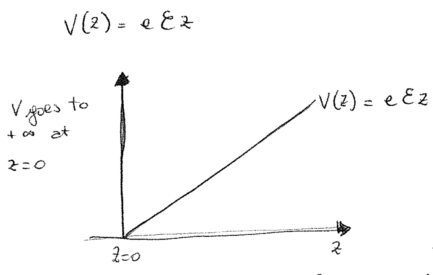
Ideal triangular potential well

Equation , on the other hand, describes the particles in a triangular potential well. The well can be approximated as a capacitor which represents the interface between the materials. The electrostatic potential associated to the uniform electric field pointing along the positive direction is:

The potential energy of an electron is

we get:

Equation is the Airy (Stokes) equation and has two possible solution and of which only the first one is acceptable ( diverges and the wave function would be non normalizable).

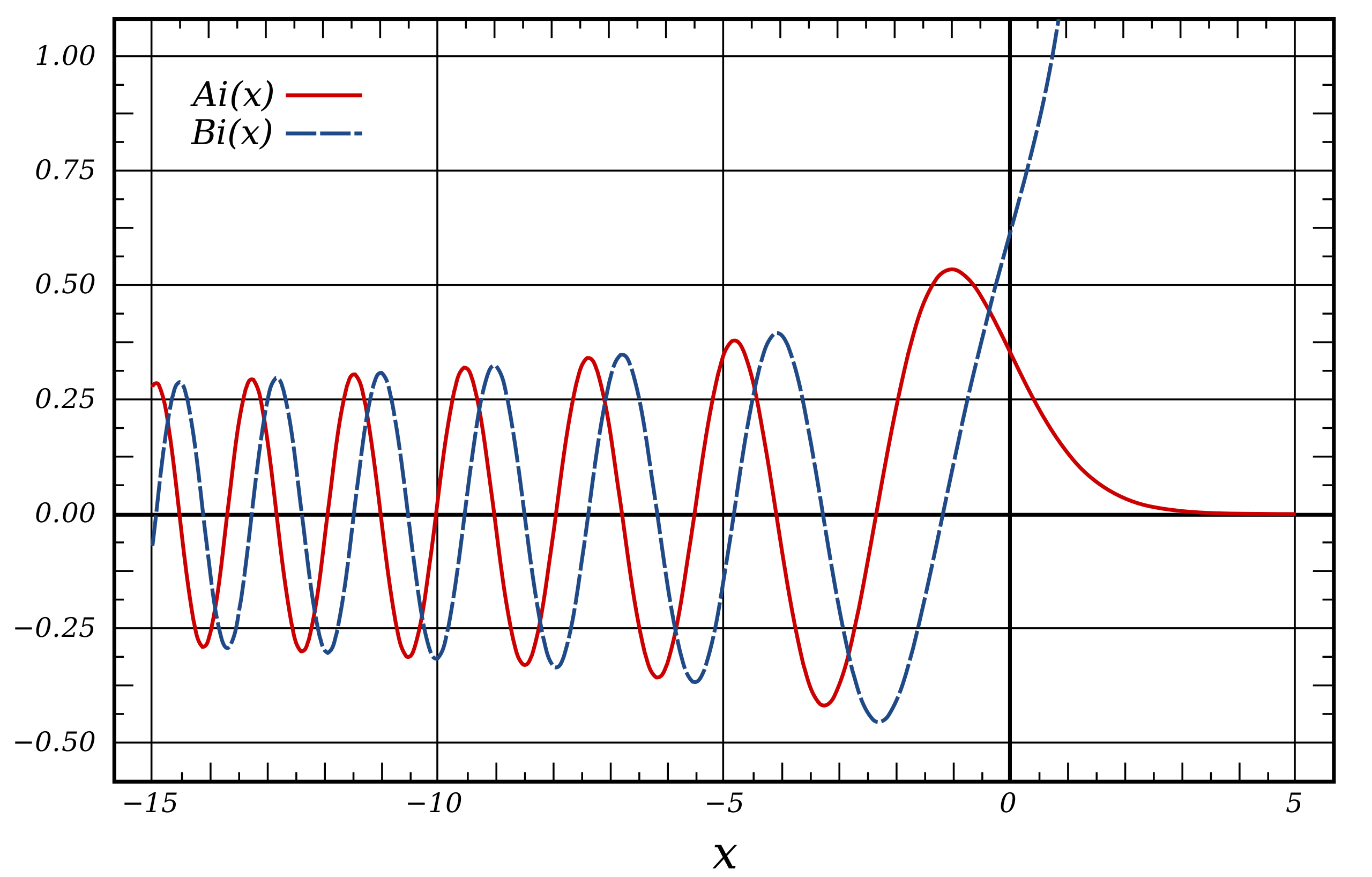
We have to impose the boundary conditions (continuity) to the SE: . Since the equation we have is in the variable we get

This is true only for the values for which . This means (similarly to the infinite potential well) that the possible energy values are quantized:

To plot the functions , since , we have to shift the plot by . Knowing the possible values of (which are the roots ), we just have to shift to the right to put in the origin and discard everything for .

For each energy level we get a different wave function.

From above we know that and thus:

Each discrete value of corresponds to an infinite number of values of . The eigenvalues are arranged in “sub-bands” one band for each value of allowed .

Density of states of a 2DEG

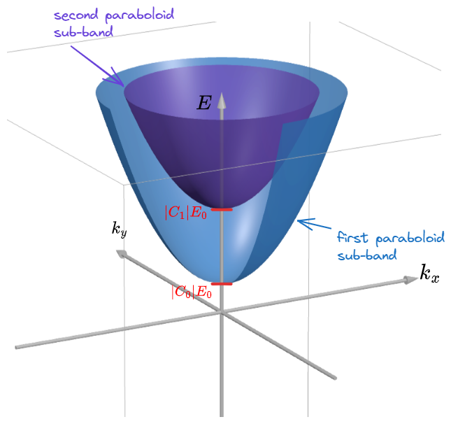
We have already seen how to calculate the density of state of electrons confined in a well; now we do it again for the energy bands generated in the 2DEG.

We can concentrate only on one band due to the fact the the DOS of the others can be calculate in the same manner. To simplify our job we start with the first band supposing that it has . Contrary to the calculation performed within the crystal, here we have only two degrees of freedom in and in and the eigenvalues are

Since we are in a 2D case, we normalize the DOS to the area, instead of the volume:

Now we can follow the same steps taken in the original case, considering that we are in two dimension and not three so we have a circle and not a sphere.

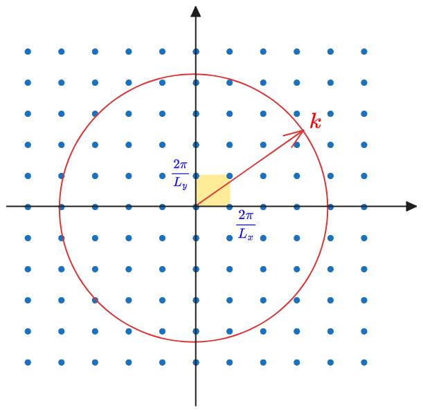
Using we can rewrite as a function of

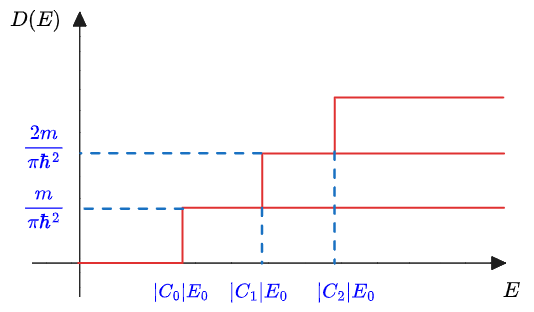
And finally, for a given sub band:

we can understand that the density of state within a subband is constant with respect to the energy.

The total density of state at any particular energy is just the sum over all the subband below that particular energy.