Fermi golden rule

Overview of the contents

Before proceeding to the main topic we should understand why it is useful and why we study it.

To study how the system evolves in this setting, we need to know the Transition Probabilities (probability of transitioning from one state to another) and the Transition rate (transition probability per unit of time) between two state and under the effect of a weak time-dependent perturbation.

Perturbation theory

The main idea behind perturbation theory is to start with a known or easily solvable system (the unperturbed system) and then introduce a small modification or perturbation that alters the behaviour of the system. By treating the perturbation as a small deviation from the known system, physicists can develop an iterative series solution where each successive term provides a more accurate approximation of the real solution.

First order perturbation

In first-order perturbation, the perturbation is assumed to be small enough that the modifications induced to the system can be linearly approximated, introducing a major simplification of the calculations. The first-order perturbation equation can be used only to approximate weak physical disturbances, such as a potential energy produced by an external field. We will use it exploring the interaction of an incoming electron with a dipole.

Results

We’ll observe that after the perturbation, the chances of the system reaching the final state are higher when the perturbation’s frequency matches that of the system. In that case we say that the perturbation is in resonance with the system and this indicates that the perturbing energy can be absorbed or emitted by the system, facilitating transitions between these states.

---

DOS

The Density of states (DOS) can be written in another equivalent form

which, differently from the one seen previously is not normalized to volume. To check that the two definition are equivalent, let’s calculate the number of state

both actions involve counting the number of energy states within the range of to , and the outcomes are identical except for a normalization factor.

Perturbation theory

Starting form a periodic unperturbed system described by the Hamiltonian the Schrödinger equation is

Supposing that the Hamiltonian is time independent we can write the solution as

When a perturbation perturbs the system, the Hamiltonian changes in

We want to find the evolution in time of the perturbed system:

we know that forms a complete basis for the unperturbed system so the general solution can be generally expressed as a linear combination:

where the coefficient are the terms responsible for the time dependance of the general solution.

Observation

The perturbation makes the system evolve from an initial state to a final state . Since each represents the probability of finding the particle in the state , after the transition (at the end of the evolution) all the coefficients will be 0 except for .

So now our goals is to calculate the coefficients and rewrite the Schrödinger equation as follows, using the Hamiltonian :

Many steps are not reported in the following.

after some steps we get:

Where

represents the matrix element representation of the perturbation between states and in the basis (solutions of the unperturbed system). The elements of the matrix can be calculated since both the perturbation and are known.

First order perturbation theory

To solve equation we need to make some assumptions: we suppose that the perturbation is so small that the system hasn’t evolved too much. So for we have and .

Indeed the FIRST ORDER APPROXIMATION consist in the assumption that:

With this approximation we can rewrite as

The transition probability (the probability of finding the system in a given (final) state ) is:

The transition rate (how fast an electron evolves from the initial state to the final state) can be calculated as:

This means that if is close to the perturbation had a strong effect on the system, so it is likely that the final state of the system after the evolution is .

Dipole in an electric field

If we imagine the perturbation generated by an incoming photon the electric field can be expressed as:

Where:

• is a complex vector representing the amplitude and phase of the electric field.
• and are the terms representing the spatial and temporal variations of the electric field due to the photon’s propagation.

We take a dipole as a system. A dipole consists of two charges of opposite polarity separated by a distance . When a photon (an electromagnetic wave) interacts with a dipole, the varying electric field of the photon exerts forces on these charges producing a perturbation.

The perturbation potential can be express as

where :

• is the electric dipole moment.
• is the value of the charges

In this case our perturbation is Now, starting from the perturbation, we will derive , the transition probability and the transition rate .

We can write for the transition from to as :

Many steps are not reported in the following.

where:

• is
• is

By plotting the first term we can see that it has a spike where (remember that ) obviously where the function makes zero. This means that the perturbation needs to have the “right” frequency () to influence the system in a meaningful way. We can also see that for short times the influence of the perturbation is smaller compared to longer times due to the factor .

Plotting the second term alone shows similar result but when . The first case corresponds to the absorption of a photon (the system increases its energy), the second one, on the other hand, to the stimulated emission of a photon.

Note that in the second case the first photon is not absorbed and only creates the perturbation, which generates the emission of a second photon

In the stimulated emission scenario, the second photon (in blue) is the emitted one, we exploit this effect in lasers.

For the function becomes so narrow that it can be approximated by

We can now calculate the , just focusing only on the first term :

todo improve

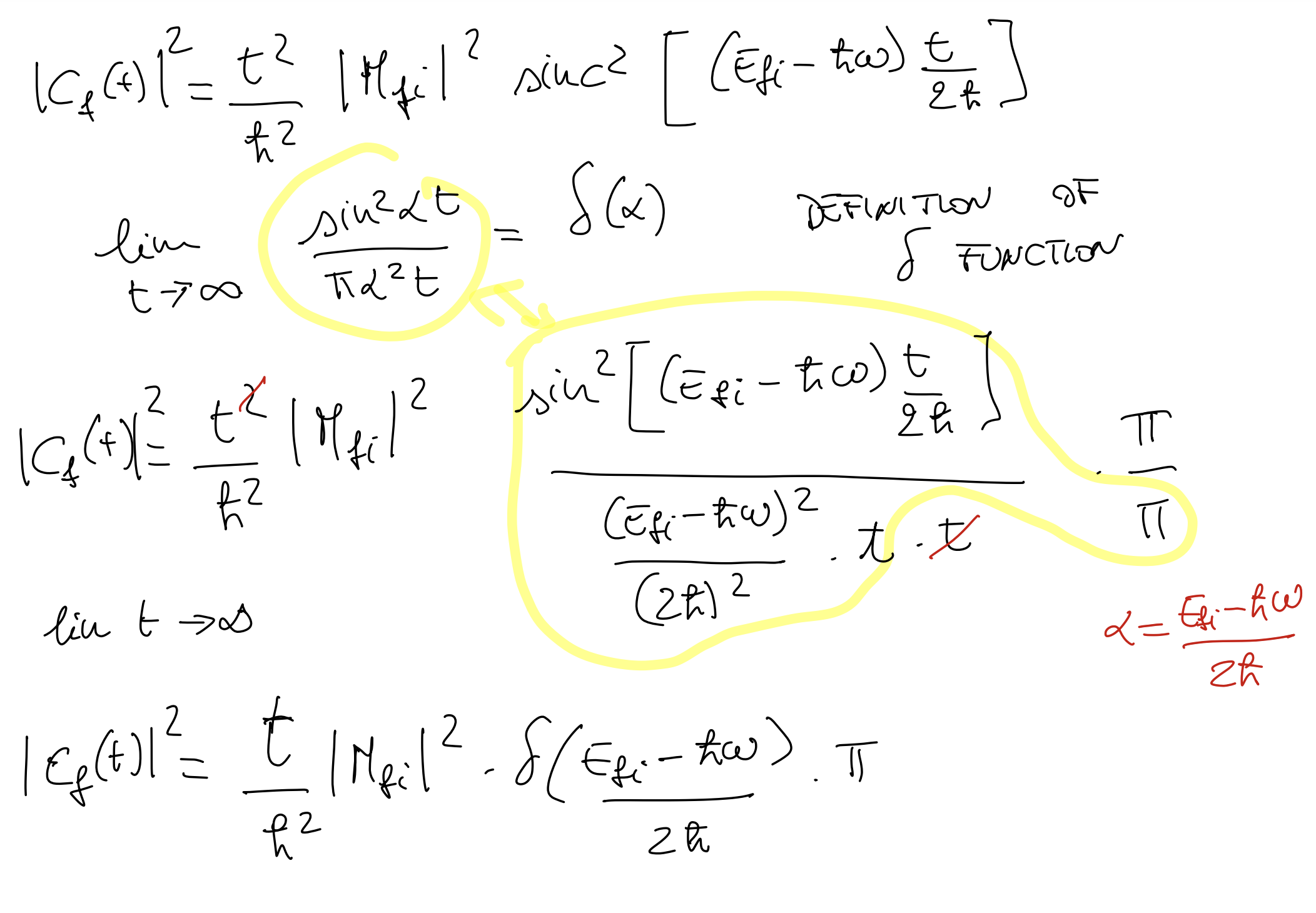
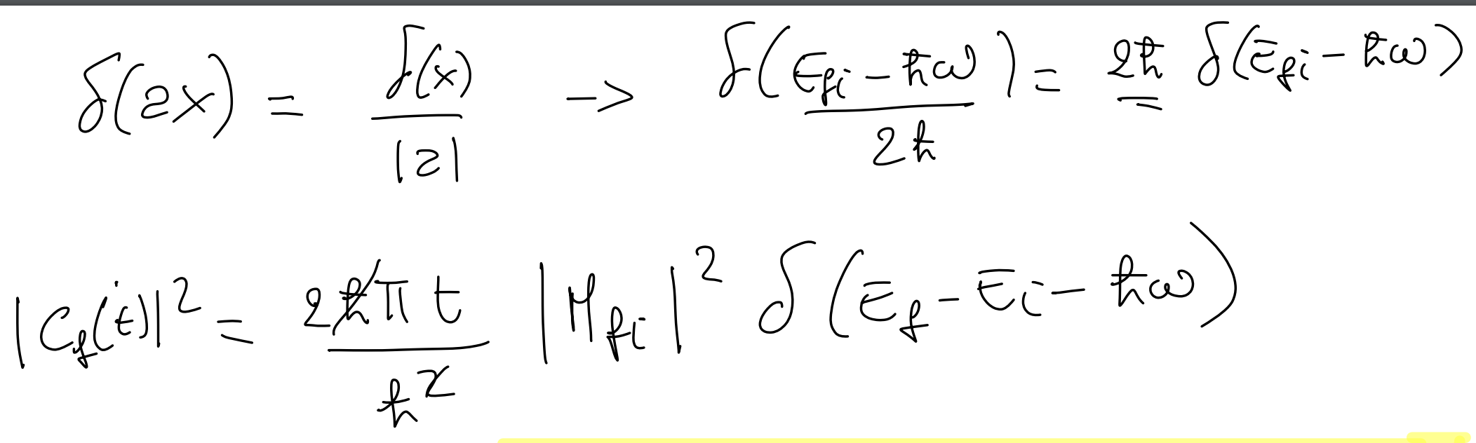
By calculating the transition rate we get the Fermi golden rule:

In Solid

In complex systems like in solid we will have multiple initial and final states that satisfy the equality and the transition will occur for each of these states.

So the formula needs to take in account the sum over all the states:

in the first step we extracted from the sum because it is non dependent from the initial and final states. Instead in the second step we replaced the sum with the definition of the Density of states (DOS).

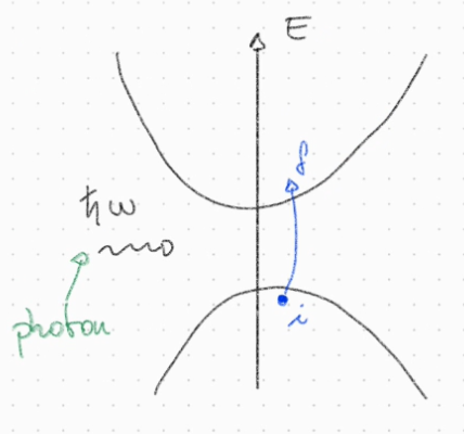
Semiconductor

todo improve drawing

Since are typically Bloch states due to the fact that we are inside a crystal structure, we can write them as:

and we can rewrite as:

When a photon is absorbed or emitted by a material, it can cause an electron to transition from one state to another.

There are two key constraints governing this transition:

• Energy conservation: The energy difference between the initial and final states is related to the photon’s energy
• Momentum conservation: The change in the wavevector caused by the transition is equal to the absorbed photon’s wavevector

• the change in momentum resulting from photon-induced transitions is negligible

So we have that:

Simplifying the electric field we get:

Since the volume of the crystal is equal to the volume of the primitive cell multiply by the number of these we can write:

We have that depends by and so it may happened that for some value of we get this case are called selection rules because in this case the transition between states is forbidden.