Quantum Hall effect

This note is based also on this lecture and this lecture suggested by the teacher

Some other references:

Kittel, page 153 Ibach Luth, Panels XIV, XV, XVI

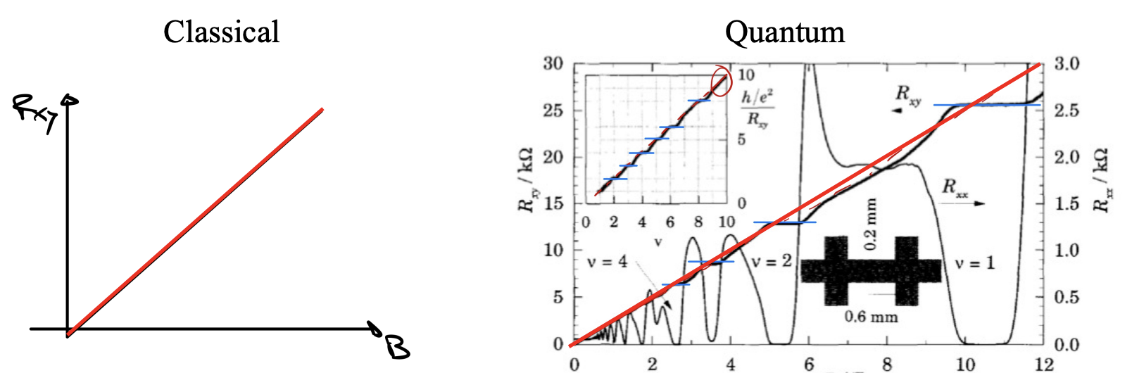
Classical case

In the classical case we have a piece of conductive material (the Hall bar in the picture below) with a perpendicular magnetic field applied. We pass a current through the bar and we measure the two voltages and (which is the Hall voltage).

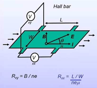
What happens to the electrons flowing in the direction is that they get deflected by the magnetic field and tend to accumulate on one side of the bar, thus creating a voltage difference in the direction. As the charge builds up, electrons will start to be subjected to a force generated by the electric field (which is opposite to the one due to ). This process will reach a stable condition when the two forces balance out and electrons will move in the direction only. This happens when

If we measure the resistance we get

Note

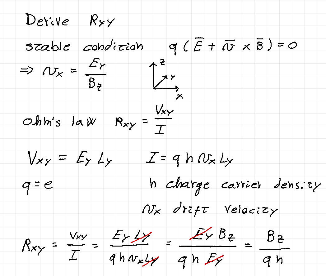
As we can see the Hall resistance does not depend on the geometry of the sample.

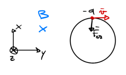
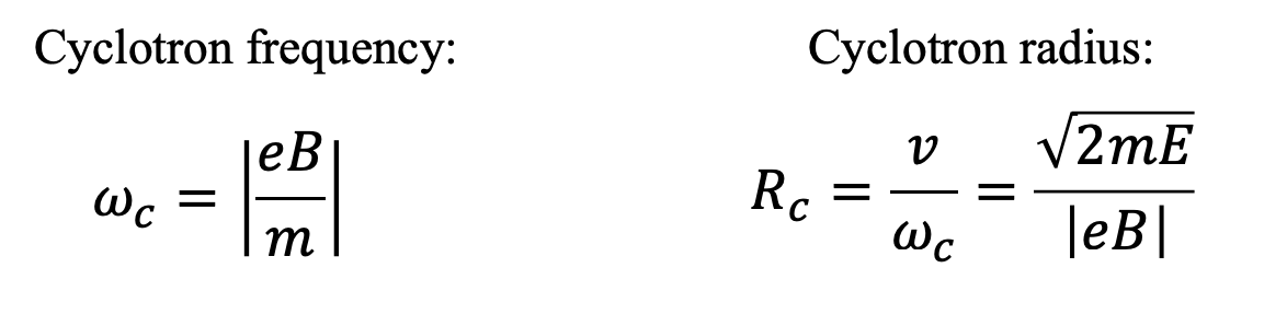
Charge in a uniform magnetic field

Before proceeding to the quantum case we need to briefly review the behaviour of a charged particle that moves in a uniform magnetic field. Supposing that the particle has an initial velocity in a plane perpendicular to the field , the particle will start moving in a circle with a radius .

Quantum case

The setup for the quantum case is similar to the previous one and can be seen in the image below.

To study what happens in the quantum case we need to solve the SE in case of both magnetic and electric fields, which is to say:

Where is the momentum component related to the magnetic field (see Vector Potential). We decide to ignore the electrostatic interaction between the charges and thus the scalar potential is .

Before proceeding we need to find a useful vector potential and we decide to use the Landau gauge that will simplify our calculations:

which is a valid choice since

By inserting the gauge in and doing the math, we get

The system that we are considering is an electron gas that is free to move in the and directions but is tightly confined in the direction. To solve this Hamiltonian it is possible to separate it into two equations since the magnetic field just affects the movement along and axes. The total energy becomes then, the sum of two contributions .

Hamiltonian directions:

The vector potential (and hence the Hamiltonian of the system) does not depend on the -coordinate. And since the Hamiltonian does not depend on , the momentum operator in the -direction commutes with the Hamiltonian. This means that ​ is a constant of motion, and its eigenfunctions are plane waves in the -direction thus we can think about the wave function as a product of a generic (unknown) function and a plane wave in the direction:

The fact that there is a “preferred direction” (i.e. the shape of the potential is not the same in the and direction) is due to the gauge we chose and not to the physics of the problem, which has a rotational symmetry with respect to the axis.

If we solve the SE with this assumption, we get

which is a quantum harmonic oscillator.

Equation of a quantum harmonic oscillator in 1D:

Comparison with the case of a uniform magnetic field:

we can see that the minima of the parabola is shifted by the value

is called the magnetic length. Since we have come back to a known case the energy levels and the wavefunctions are easily derived:

With

The energy states, are called Landau levels, these levels are highly degenerate (many electron states have the same energy). Indeed, from the expression one notices that the energy depends only on , not on , so states with the same  but different  are degenerate.

We observe that the value of is influenced by the parameter , which must be determined by solving the Schrödinger equation in the direction (infinite potential well). It’s important to note that is not a continuously varying parameter but is quantized. We can obtain these quantized values by applying periodic boundary conditions, from which we derive the following relationship:

Now we know how distant the parabolas are from each other. There are oscillators in every

Number of harmonic oscillators

Since our sample has finite dimensions, the number of harmonic oscillator must be finite as well. This number can be calculated as follows:

varies between and so we can write

which can be rearranged to find the range of variation of :

Finally, can be calculated as the ratio between the total range of variation of and the distance between two :

we can also calculate as the ratio between the (magnetic) flux through the sample divided by the minimum flux of a single state the quantum of flux

Landau levels

Due to the fact that the harmonic oscillator has discrete energy levels with a spacing of we can easily draw the density of states:

todo image doesn’t render on the website for some reason

The “height” (density of states per unit surface) of the Landau levels can be easily determined as

​ gives the density of states, which is the number of available quantum states for the electrons at each energy level per unit area. In a strong magnetic field, the electron’s motion perpendicular to the field is quantized into Landau levels. The formula shows that as the magnetic field strength increases, the density of states at each Landau level increases, meaning more states are available for electrons at each quantized energy level.

Recap

From what we saw so far, we noticed that we have a series of harmonic oscillators that spread along the direction. Since all the harmonic oscillators have the same energies, there will be a number of degeneracies equal to the number of harmonic oscillators .

Dependence on

As we increase the magnitude of the magnetic field, we are changing the degeneracy and the distance of the Landau levels (check the video below)

source

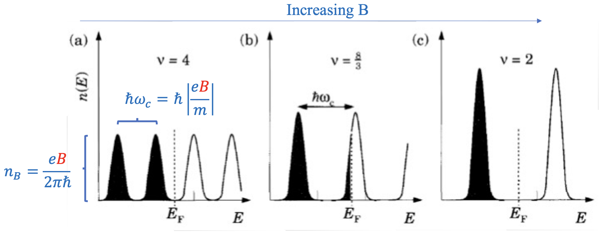The larger , the more degenerate the levels are and the further apart they are.

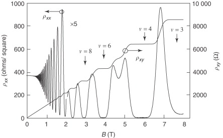
Shubnikov - de Haas effect

When a current is applied between two electrodes in a 2DEG exposed to a magnetic field the measured resistance along the direction is found to oscillate. This is called the Shubnikov-de Haas effect. ()

Landau level filling

The filling factor of a Landaus levels, is a factor that tell us how many Landau levels are filled by electrons per unit of area. Since each Landau level has an associated density of state , the factor can be written as:

where is the electron density of the 2DEG.

If we keep the constant and the magnetic field is increased, the Landau level filling changes.

Certainly, when we increase the value of , the quantity also increases. If we maintain at a constant level, this implies that the factor must decrease.

When the filling factor is an integer the 2DEG does not conduct electricity.

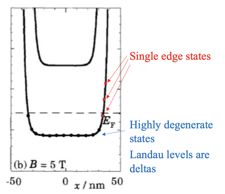
Effect of edges

We must take into account the impact of the edges on the energy of states within the Landau levels. When approaching the edge, the electron’s orbit is subject to perturbations.

From a semiclassical point of view we can say that due to these perturbations, the frequency of oscillation increases, resulting in shorter orbits. Since frequency and energy are directly linked, it’s intuitive to conclude that the closer an electron is to the surface, the higher its energy states will be.

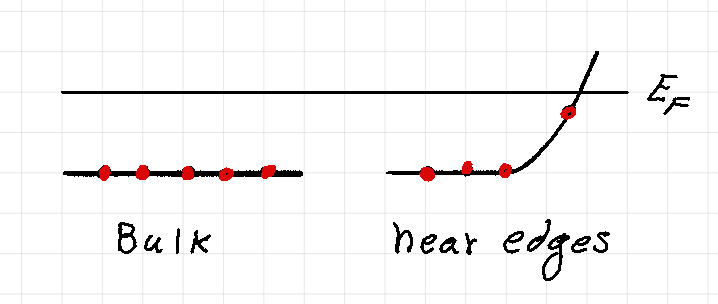
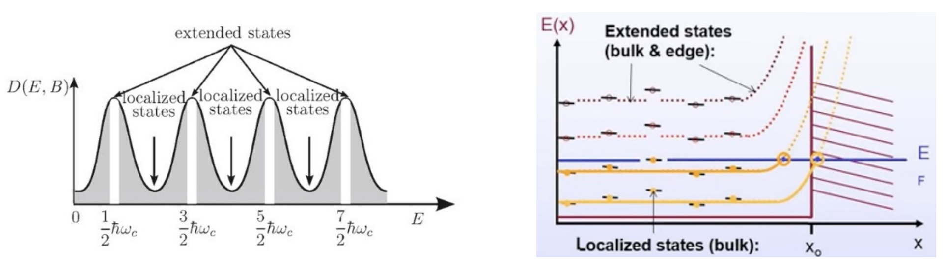
By solving the Schrödinger equation and substituting the potential with an infinite potential at the material’s edges, we find that states located in the middle of the material, characterized by small values of , remain unaffected by the presence of the edges. This validates the solutions obtained earlier. On the other hand, states near the material’s edges, corresponding to large values of , experience compression within a narrower space, resulting in higher energy levels.

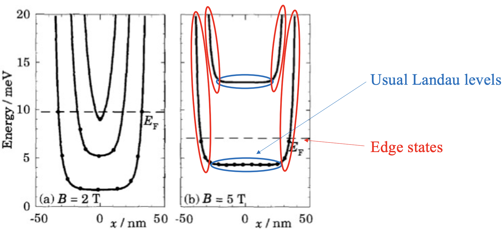
When the Fermi level falls between two Landau levels, the bulk does not conduct as all states within this range are filled. However, at the edges, there are conducting states due to the increase in energy near the edges

Effect of impurities

In real materials, there are always some impurities and phonons that can scatter electrons. This effect introduces an uncertainty in the energy, we can describe this uncertainty expanding the delta-like Landau levels into Gaussians characterized by a full width at half maximum

In which is the average time between two scattering events (lifetime of the electron)

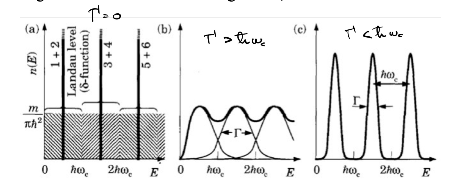
In a perfectly pure material without any impurities (where , the broadening of the energy levels, is zero), Landau levels are highly degenerate and sharply defined. Edge states, on the other hand, are not degenerate.

When the magnetic field () is varied in such system, the edge states immediately get occupied with electrons as they are available. Since the material is pure and there is no energy level broadening ( = 0), the Fermi level jumps directly from one fully occupied Landau level to the next as the magnetic field changes. There’s no smooth transition or plateau.

Origin of plateaus in QHE

In the real world, however, materials are not perfectly pure and contain impurities. These impurities cause the energy levels to broaden ( > 0), which means the energy levels are not as sharply defined. This broadening is created by impurities, that are localized so the states in the broadened regions don’t contribute to the overall current and this has the effect to ‘pin’ the Fermi level between the Landau levels as the magnetic field changes. Rather than the Fermi level jumping sharply from one level to the next, it gets stuck in these broadened areas for a range of magnetic field values.

Because the Fermi level is pinned, as we vary the magnetic field, we see plateaus in the . These plateaus occur where the Fermi level is in the broadened region due to impurities.

So, the plateaus in the Hall resistance that are characteristic of the Quantum Hall Effect are actually a consequence of the Fermi level being pinned between Landau levels by impurities in the material. Without these impurities and the associated broadening, there would be no plateaus—just sharp transitions as the magnetic field changes.

To shows the plateaus in the graph we need to rewrite the resistance in another form. Recalling from the from the classical Hall effect:

Now remembering the definition of the filling factor and the definition of quantum of flux:

we get the quantum Hall resistance:

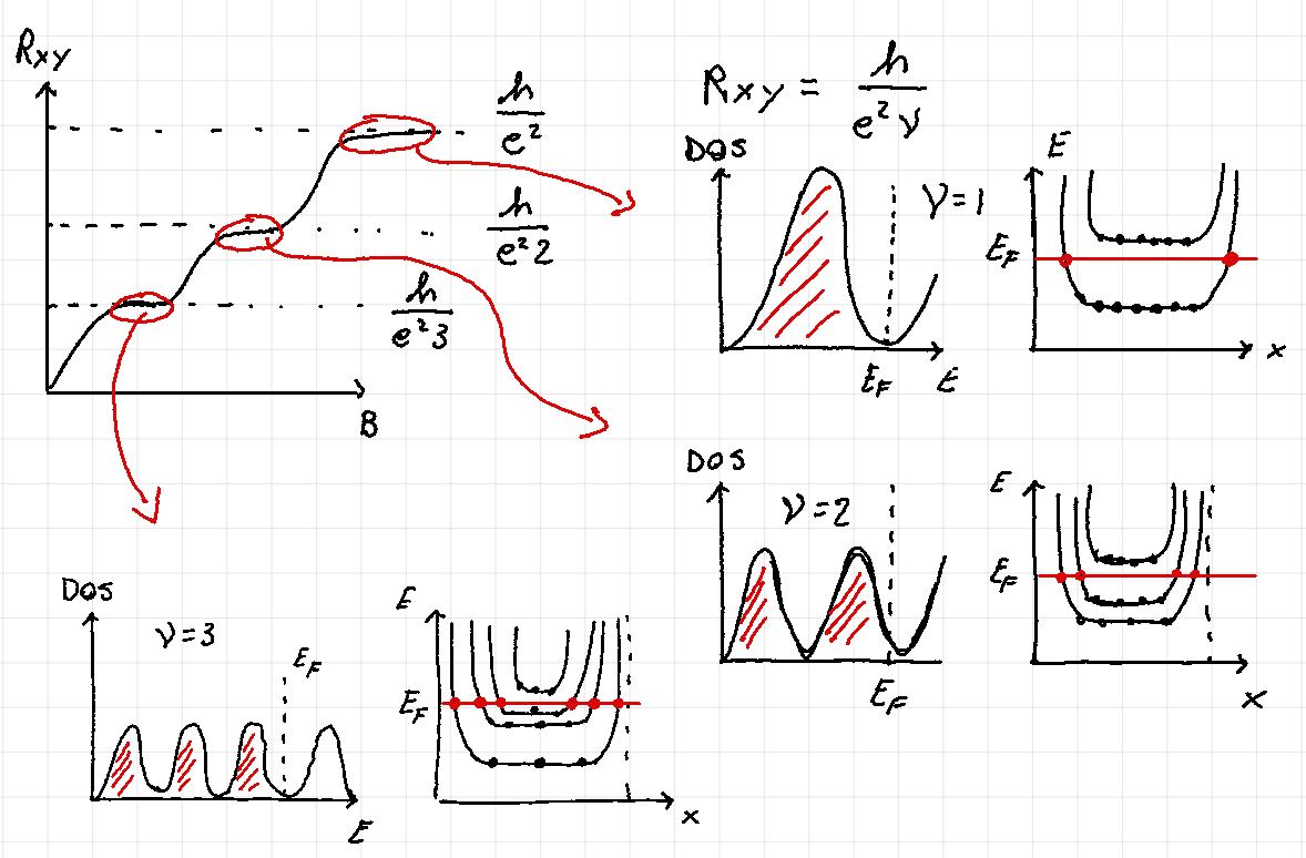
The are plateaus in the Hall resistance even when the filling factor is not an exact integer due to the presence of localized states caused by impurities and disorder in real materials.

QHE at the device level

At the device level, edge states leads to QHE as follows

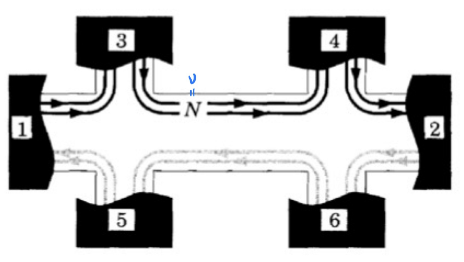
A potential difference is applied between electrode 1 and electrode 2 to drive a current through the device. The electrons travel from electrode 1 to electrode 2. However, due to the magnetic field (not shown in the figure, but perpendicular to the plane of the device), the electrons will follow edge states that are at the boundaries of the sample.

The electrons leaving 1 will first enter in 3 and then in 4 (3 and 4 are not allowed to draw current) so that , For the same reason: .

Since we place we have that and thus a Hall resistance is measured between 3 and 5 or 4 and 6.