Free electron model

Where Ibach Luth is mentioned we refer to

Ibach Luth Solid-State Physics An Introduction to Principles of Materials Science Fourth Edition

In this chapter we will deal only with the “outer” electrons, since the inner ones behave similarly to the isolated atom.

The complete SE for one electron is

where are the positions and the spins.

We will always assume the following two approximations:

1. Born/Oppenheimer (adiabatic) approximation: electrons and nuclei are decoupled
2. Independent electrons

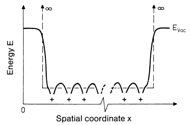
In the free electron model, we will also assume that the electrons are free, which means that the potential is 0 everywhere.

Sommerfeld - Bethe model

This should correspond to the free and independent electron model from condensed matter

This simpler model is useful when the electrons are loosely bound, such as in metals. The electrons are considered to be confined in box of edge with infinite potential barriers at the edges and a constant potential inside.

We will consider the case at and with electrons.

The SE will be

with

The boundary conditions are the Born - Von Karman or periodic boundary conditions:

Boundary conditions explanation omitted

By solving the SE we get that the solution is a plane wave:

The normalization constant can be calculated by imposing

where is the volume of the cube.

Energy eigenvalues

Boundary conditions

The BVK conditions are satisfied by imposing each of the three conditions . Doing this for the first one results in:

which means that the exponential has to be equal to and thus

The same is true for and :

Notice that since is a macroscopic value, the s are quasi-continuous.

Density of states

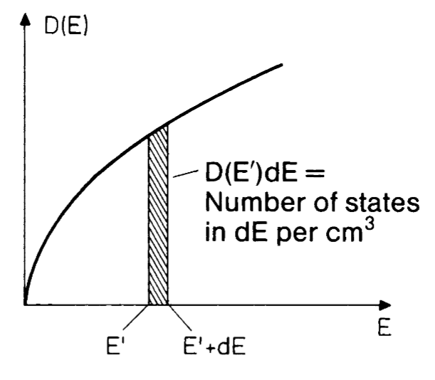
The density of states is defined as the number of electronic states per unit energy and unit volume:

The volume of the single state (in green) is given by .

If we define as the generic volume in k-space then the number of states is given by

Because of the spin degeneracy, each state contains two electrons, thus:

Remembering the value of the energy and obtaining from it, we get

Calculating the DOS from we get:

Finally, the DOS for the free electron gas is

todo pagg 16/17 bianco ???

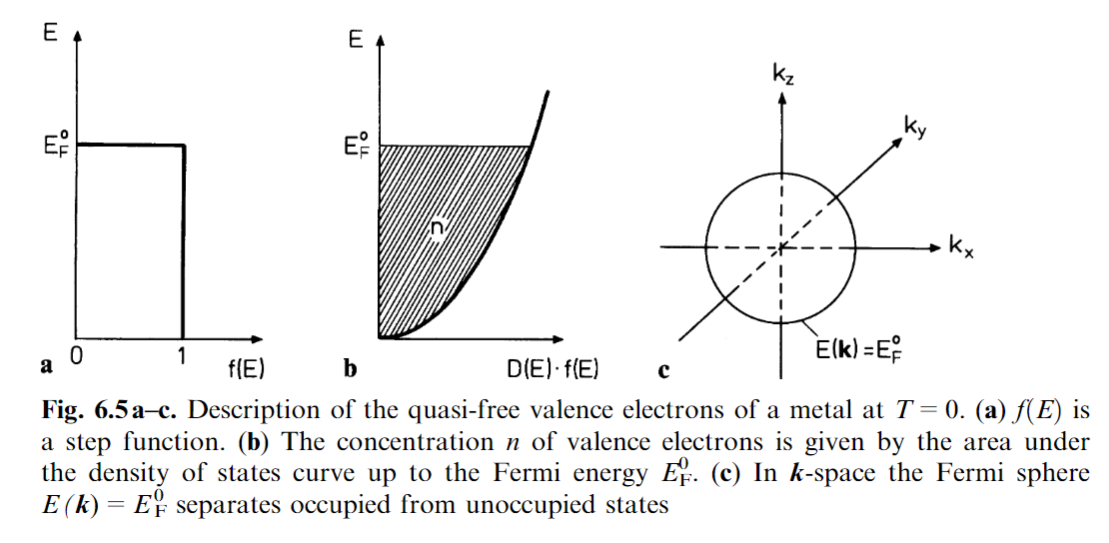
Energy of Fermi gas @ T = 0K

Ibach Luth, 6.2

The internal energy density can be calculated as

In we used the fact that (todo where does it come from?).

From this we can see that, as a consequence of the Pauli exclusion principle, even at the energy of the gas is non zero.

Since is orders of magnitude higher than the internal energy of a classical gas (Boltzmann) at , we can study the conduction electron gas regardless of the effects of the temperature.

Density of states: general formula

Fermi gas @ T > 0K

What we want to do now is estimate the width of the region where the Fermi-Dirac varies.

Ibach Luth, 6.3

If we impose and , this can be done by approximating the slope with the tangent line in and calculating the intersections with and .

From the equation of the straight line we need to find:

and, since :

We finally get:

If we calculate the interceptions with the two horizontal lines and we that they are located at:

and so the range where varies is equal to which is much smaller than , so:

Which is a classical Boltzmann distribution

Thermal properties in classical gas

The internal energy of a classical gas of particles is

and its internal energy density is

The specific heat is given by

Thermal properties in metals

Ibach Luth, 6.4

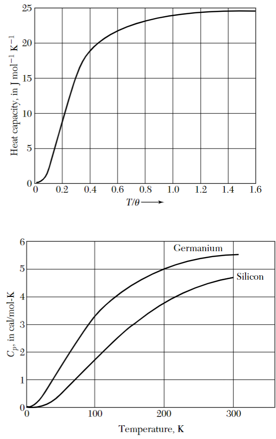
From what we just saw, we would expect that the specific heat of the electron gas would increase linearly with the number of electrons but experiments show that this is not the case. What we observe is that metals follow the Dulong-Petit law, where the specific heat tends to a constant value as temperature increases.

The reason is simple: electrons, in contrast to a classical gas, can only gain energy if they can move into free states in their energetic neighbourhood. Looking at what we saw before, this can be expressed as the fact that the electrons that can “move” are only the ones in the region , which is much smaller that .

We now want to show that the specific heat of the electrons is negligible compared to the one of the lattice.

To do this we want to calculate of the electrons. First of all we need the increase in internal energy density

Where the second integral is the density of internal energy at

From the definition of specific heat, deriving we get

In order to simplify the calculation we can exploit the following relation:

E_{F}\cdot n = E_{F} \int_{0}^{\infty} D(E)f(E,T) , dE \tag{6} $$

Subtracting from , is obtained as:

Focusing around , because the electron can only gain energy if they can move into free states in their energetic neighbourhood, we can see that the is nearly constant in the range and can be approximated by

and the derivative of the Fermi function is:

substituting in

c_{v}=Tk_{B}^{2}D(E_{F})\int_{-\frac{E_{F}}{k_{B}T}}^{\infty} \frac{x^{2}e^{x}}{(e^{x}+1)^{2}}, dx \tag{11}

c_{v}=Tk_{B}^{2}D(E_{F})\int_{-\infty}^{\infty} \frac{x^{2}e^{x}}{(e^{x}+1)^{2}}, dx \tag{12}

\int_{-\infty}^{\infty} \frac{x^{2}e^{x}}{(e^{x}+1)^{2}}, dx=\frac{\pi^{2}}{3} \tag{13}

c_{v}\simeq Tk_{B}^{2}D(E_{F})\frac{\pi^{2}}{3} \tag{14}

n=\int_{0}^{E_{F}}D(E) , dE \tag{15}

\displaylines{ D(E)=D(E) \frac{E_{F}^{1/2}}{E_{F}^{1/2}} =\ =\frac{m}{(\pi \hbar)^{2}} \left( \frac{2m}{\hbar^{2}} \right)^{1/2} E_{F}^{1/2} \frac{E^{1/2}}{E_{F}^{1/2}} = D(E_{F})\left( \frac{E}{E_{F}} \right)^{1/2} \tag{16} }

D(E_{F})=\frac{3}{2} \frac{n}{E_{F}} \tag{17}

c_{v}=\frac{\pi^{2}}{2}nk_{B} \frac{T}{T_{F}}

c_{v}=\gamma T+\beta T