Quantum Dots

In a quantum dot we have

We have 3 dimension of confinement and zero degree of freedom for electrons.

We are able control the amount of charge in a quantum dot connecting the dot to electrodes.

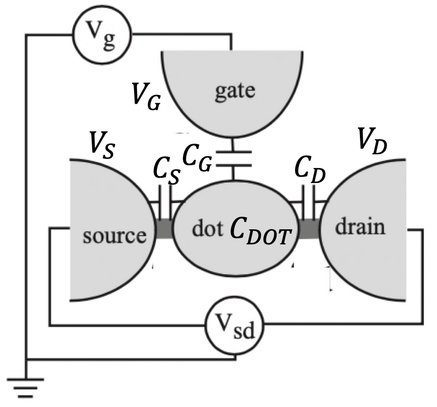
The dot can be coupled via tunnel barriers to reservoirs (source and drain), with which electrons can be exchanged. The dot is also coupled capacitively to a gate electrode, which can be used to tune the electrostatic potential of the dot with respect to the reservoirs.

Constant Interaction Model

In quantum dot systems, particularly when studying charge manipulation, the Constant Interaction Model is often employed as a simplifying approximation. This model helps to understand the electronic properties of quantum dots, especially when dealing with Coulomb blockade and single-electron tunneling phenomena. The Constant Interaction Model relies on two key approximations:

1. Constant Capacitance Assumption: This approximation assumes that the Coulomb interactions among electrons within the quantum dot, as well as between the electrons in the dot and those in the environment, can be parameterized by a single, constant capacitance value. This means that the charging energy of the quantum dot, which is the energy required to add an additional electron to the dot, is considered to be constant, regardless of the number of electrons already present in the dot. Under this approximation, the energy required to add each additional electron is the same, leading to equally spaced addition energy levels.

2. Independence of Single-Particle Energy Levels from Interactions: The second approximation is that the single-particle energy-level spectrum of the quantum dot is independent of the Coulomb interactions and, therefore, of the number of electrons. This approximation simplifies the theoretical treatment by treating the quantum dot as a simple potential well where the energy levels are determined by the dot’s size and shape, independent of its charge state.

Charge manipulation in quantum dots

We want to calculate the charge on the dot as function of the applied voltages on the electrodes. Recalling that

we start writing:

this formula leads us to:

We are, interested in the electrostatic energy variation induced by the addition of electrons to the base amount of charge in the dot, so we need to integrate the potential by the charge:

Note so we can write the electrostatic potential as function of the total amount of charges.

The electrostatic energy is summed up to the single electron energy in QD to find the total energy of the system:

The total energy of the quantum dot system with electrons is the sum of the electrostatic energy and the energies of all the occupied single-electron states.

the electrochemical potential , is a thermodynamic measure of chemical potential that does not omit the energy contribution of electrostatics and we can use it to describe the total energy cost to vary the number of electrons by one:

Substituting we get:

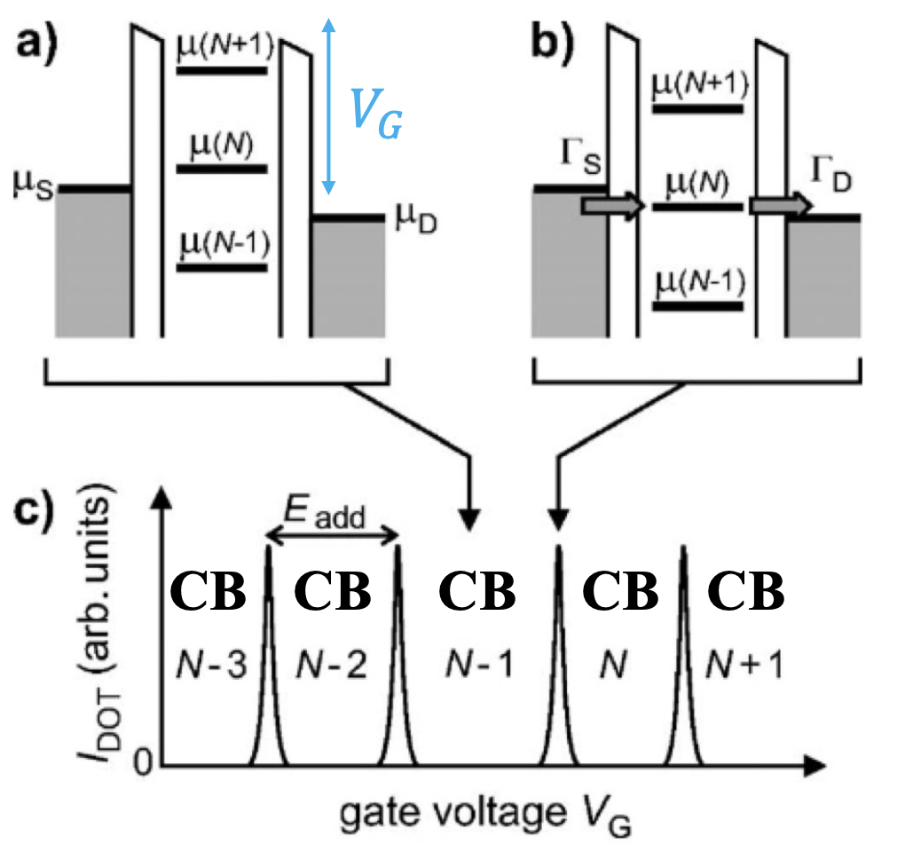
The electrochemical potential depends linearly on the gate voltage, The effect of is to shift the energy level of the dot with respect to the source and drain.

The electrochemical potential gives an indication of the energy requirements to add electrons to the dot. When the electrochemical potential does not match the energy provided by the gate voltage, electrons cannot tunnel through the quantum dot, effectively blocking the current - this is the Coulomb blockade. By adjusting the gate voltage, the energy levels within the dot can be tuned until they align with the source and drain, allowing electrons to tunnel through, and current to flow

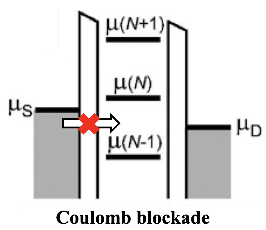
To unblock the dot, one must act on the applied voltages, either increasing the or shifting the levels with .

There are two main regimes of application of a : low bias and high bias.

1. Low Bias 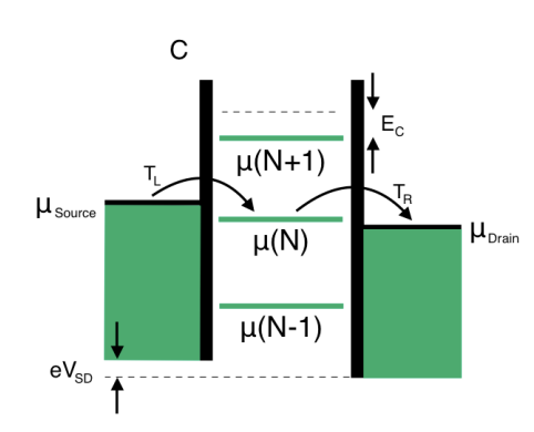In the low bias regime, at most one level is within the bias window. By definition, in the low-bias regime considered here, no excited states exist.

2. High bias

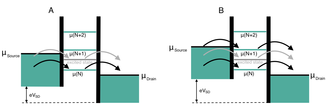
In the high bias regime, multiple levels can be within the bias window.

Electron transport is only possible when a level is in the bias window, i.e., ≥ for at least one value of . When the electrochemical potential is in the bias window, one extra electron can tunnel onto the dot from the source, so that the number of electrons increases from to , after it has tunneled to the drain, another electron can tunnel onto the dot from the source. This cycle is known as single-electron tunneling.

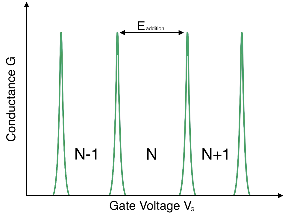
Coulomb blockade diamonds

Low Bias

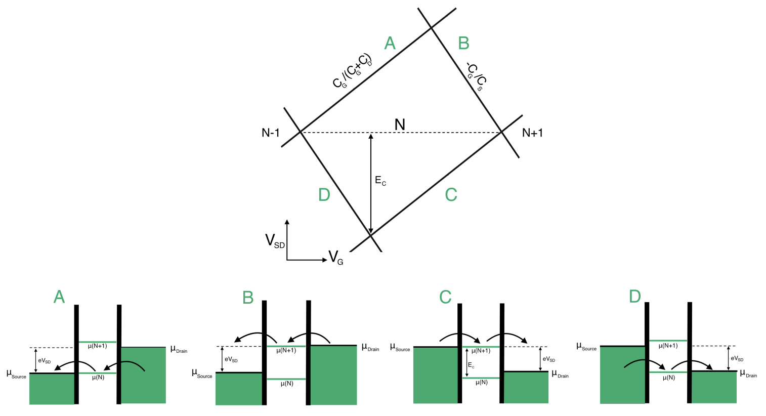
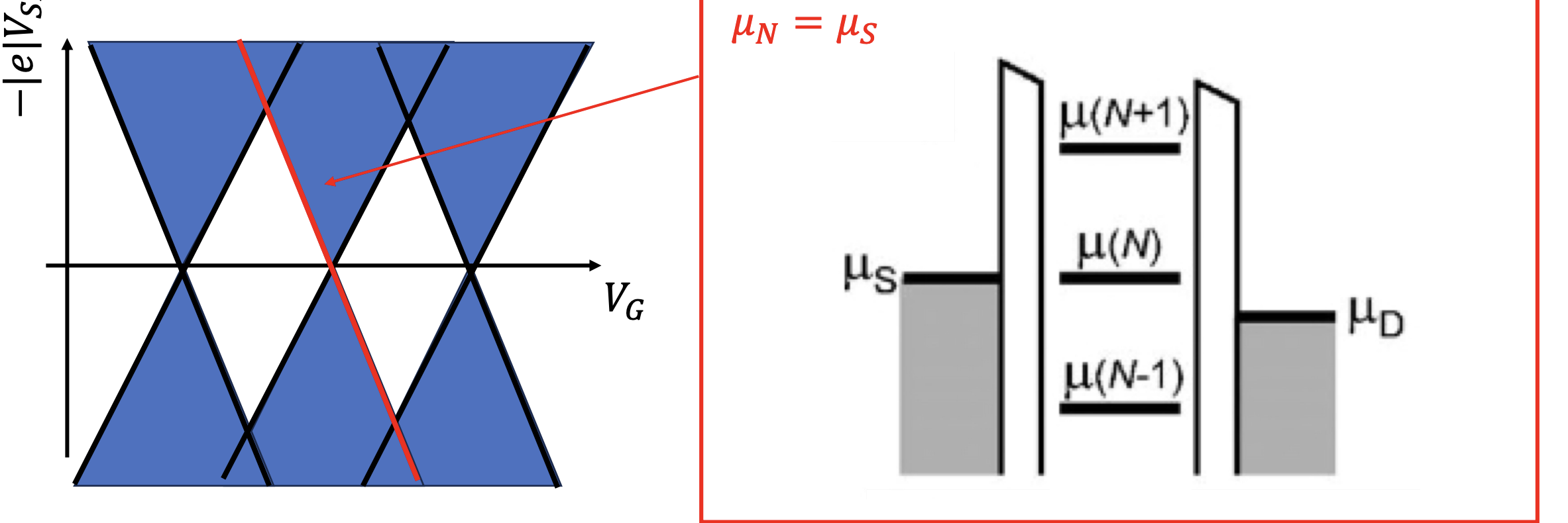
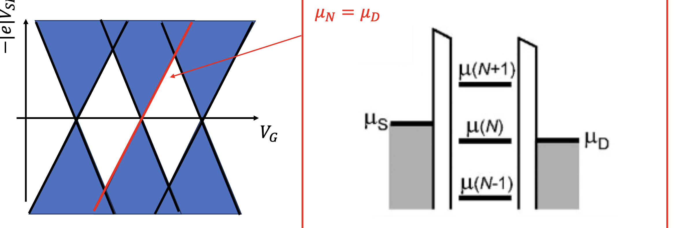
A source-drain bias voltage versus gate voltage plot can be made. This plot is often called a level spectroscopy diagram or a stability diagram and always exhibits a characteristic rhombic structure. Inside the diamond-shaped regions, the number of electrons on the dot is fixed due to the Coulomb blockade effect and no current can flow through them. These regions are often called Coulomb diamonds. Each diamond corresponds to a fixed number of N electrons inside the dot. The points at the end of each diamond where the upper right and lower right edge of the diamond join along the gate voltage axis are called degeneracy points. At these points the energy of adding the and the electron to the dot is the same (thus, the characterization “degenerate”). Outside the diamonds, the Coulomb blockade is lifted and single-electron tunneling events and thus current flow, take place. The edges of each diamond therefore signify the onset or the termination of a current flow. As we move to the right of the plot, there is a higher gate voltage and therefore the electrochemical potential “ladder” on the dot shifts down. Every time the edge of a diamond is reached, there is an alignment between one of the the electrochemical potential levels inside the dot and the electrochemical potential level of either the source (upper left and lower right diamond edges) or the drain (upper right and lower left diamond edges).

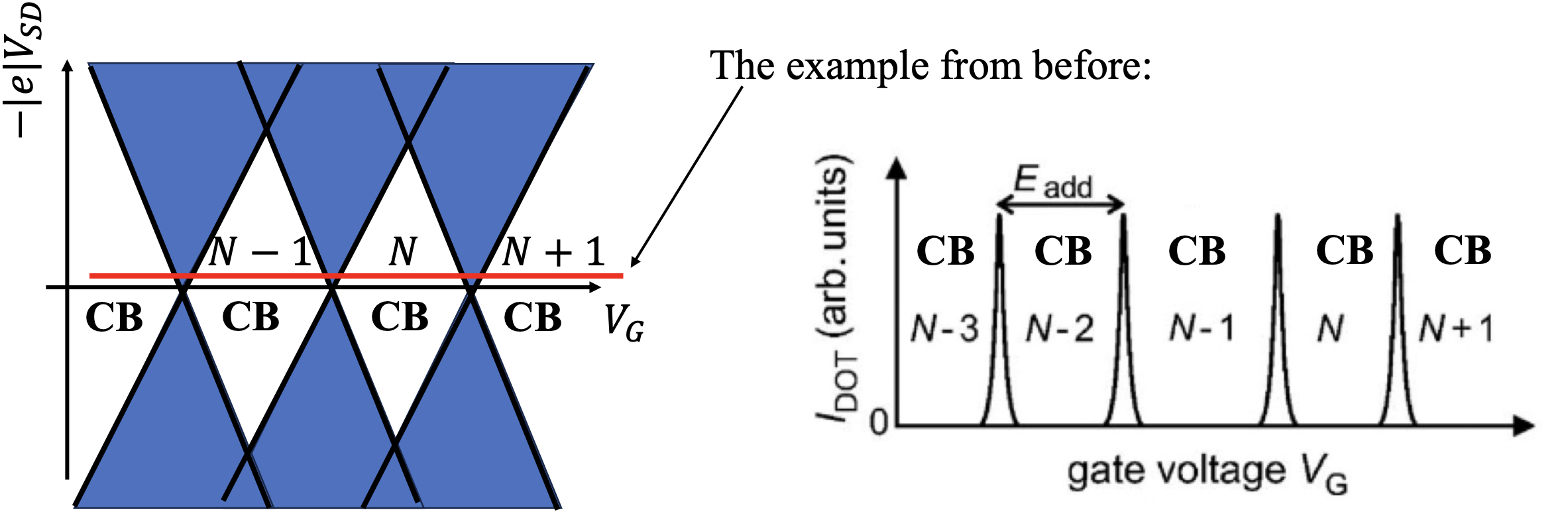
The shape of the Coulomb diamonds can be interpreted as follows:

If we assume that the bias is applied symmetrically so the voltage is applied in such a way that the source’s energy is increased by half the applied voltage , and the drain’s energy is decreased by the same amount. When no voltage is applied (), the energy levels of the source and the drain are equal (denoted as ​). Now, the stability of an electron configuration inside the quantum dot is determined by comparing the electrochemical potential of the quantum dot with the modified energy levels of the source and drain due to the applied voltage. For electrons to move into the quantum dot (for positive ​), the quantum dot’s electrochemical potential must be higher than the drain’s and lower than the source’s. For electrons to move out (for negative ​), the opposite is true. These conditions can be written as a set of inequalities that determine when the quantum dot is stable (no electrons can move in or out, leading to what we call the Coulomb blockade) or unstable (electrons can move, lifting the Coulomb blockade). When you plot these conditions on a diagram of current versus voltage, the regions where the quantum dot is stable (Coulomb blockade) form shapes that look like diamonds.

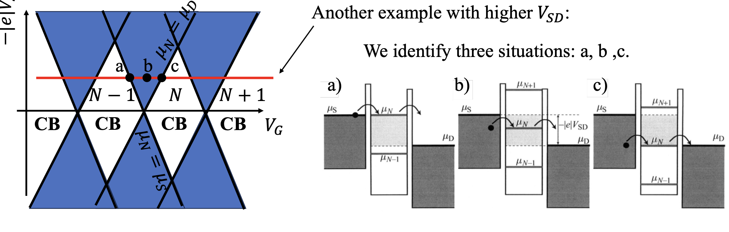
High Bias

At the high bias regime, multiple dot energy levels can participate in the charge tunneling. Every time an excited state level enters the (now widened) bias window together with an electrochemical potential level in the dot, an additional transport channel opens up allowing electrons to tunnel via one of the two levels. Also, multiple tunneling events can take place at the same time if multiple electrochemical potentials are aligned inside the bias window. The new transport channels due to the excited states appear in the stability diagram discussed earlier as lines running parallel to the diamond edges:

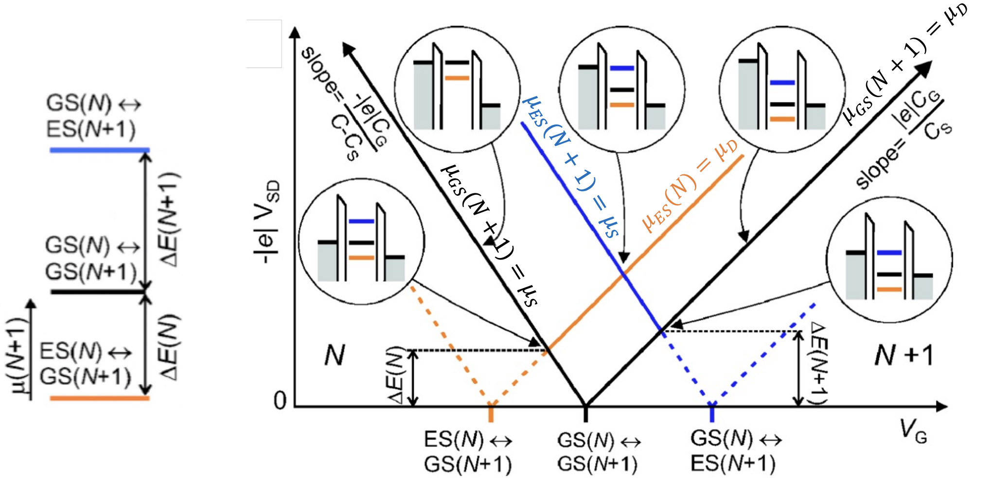
The plot describe transport with the same Coulomb blockade diamonds. This time accounting for the additional excited states.

Excited states (ES) can arise from a number of reasons. For example If a magnetic field is applied the spin up and down states are no longer degenerate but they split in energy due to Zeeman effect.

Interaction between QDots

In a similar to a single quantum dot fashion, systems consisting of two coupled quantum dots can be fabricated. Where single quantum dots are regarded as artificial atoms, coupled double quantum dots can be considered as artificial molecules

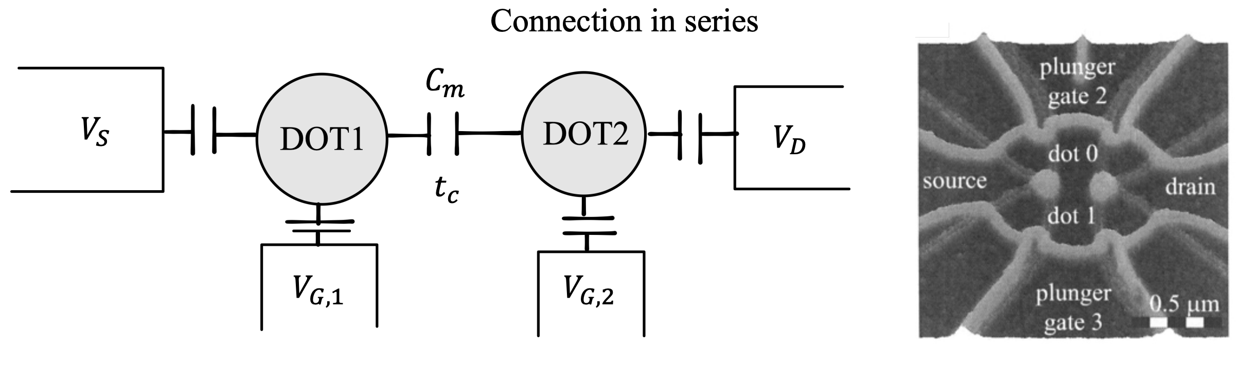
Usually, two contributions to the coupling have to be considered:

• The electrostatic interaction between the electrons of neighboring dots (capacitive coupling)
• The possibility of electron tunneling between dots (tunneling coupling)

Capacitive coupling

The capacity coupling is modelled by a capacitance term (mutual coupling capacitance), indicating the strength of interaction between charges of the two dots.

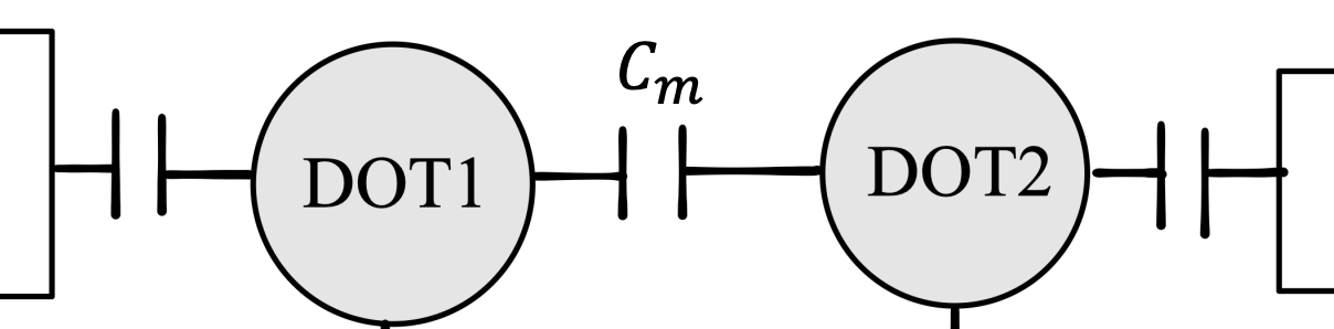
For large distances, the electrostatic interactions between dots are negligible so .

In this case, the amount of charge on one node is not influenced by the other.

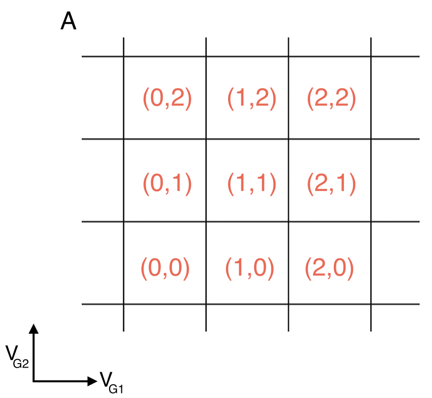
Stability diagrams for double quantum dot systems. Inside each domain the charge is constant, while on the edges of the border lines between the domains, charges can flow. The lines indicate the gate voltage values at which the number of charges changes. The number of charges on each domain is denoted by (N1,N2). These diagrams can be viewed as an extension in two dimensions of the coulomb peak diagram presented in figure

In A, the capacitive coupling between the two dots is negligible, making the two dots effectively independent.

For smaller distances, the electrostatic interactions between dots become significant

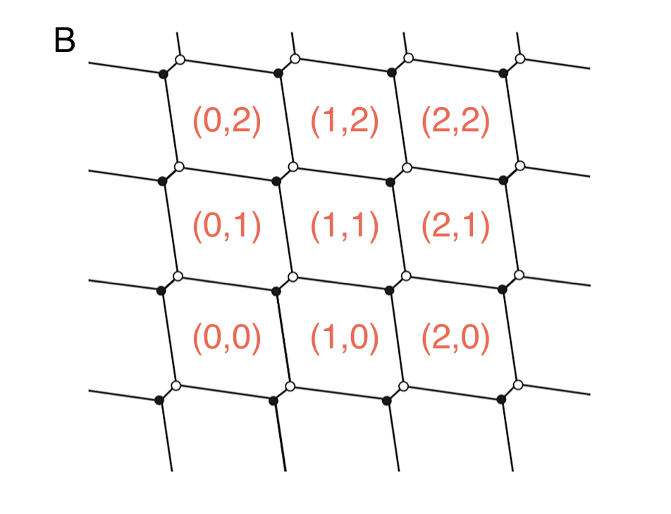
When the mutual capacitive coupling between the dots ​ is greater than zero, it means that there is significant electrostatic interaction between the two quantum dots.

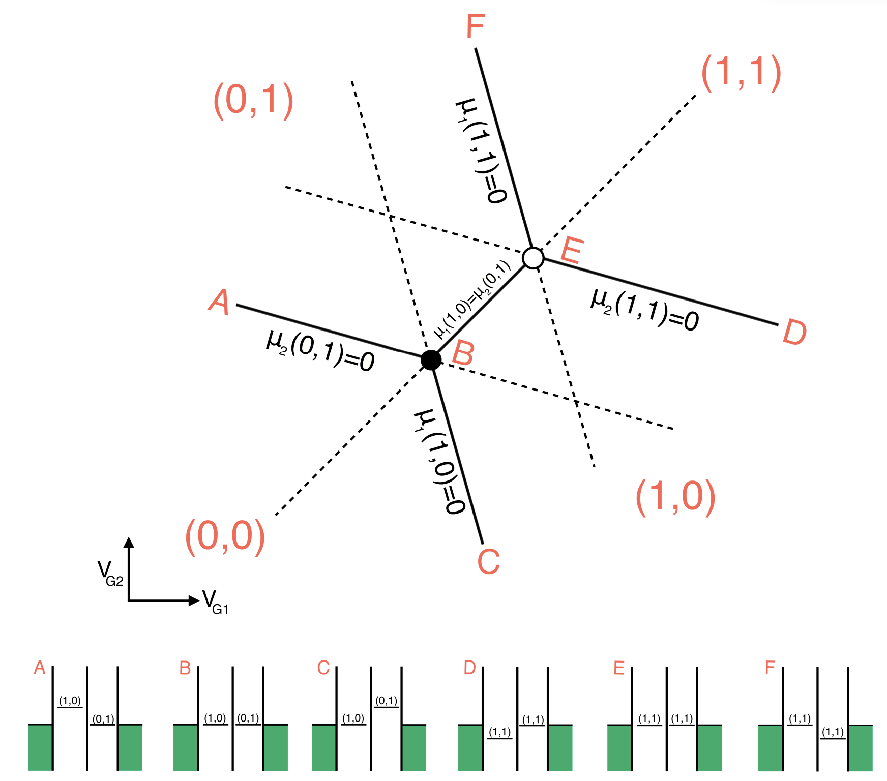
Triple Points: At certain gate voltages, the electrochemical potentials of the two quantum dots align with the source and drain, allowing electrons to tunnel onto and off the dots. These gate voltages correspond to the vertices of the honeycomb pattern and are called “triple points” because three different charge configurations are energetically degenerate. Only on these points, a current can flow from source to drain.

Focus on the triple points:

Tunneling coupling

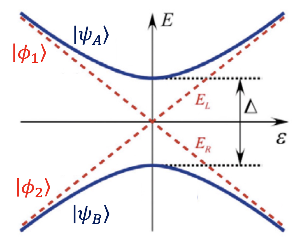
When distances are small, tunneling between dots can occur. Much like superlattices, this leads to a change in the levels of the dots. In superlattices we had a periodic structure. Here, instead, we only have two dots. The configuration recalls the one of a molecule made of two atoms.

Therefore, because of the tunneling coupling (), bonding and antibonding orbitals arise from the combination of the two dots levels ( and )

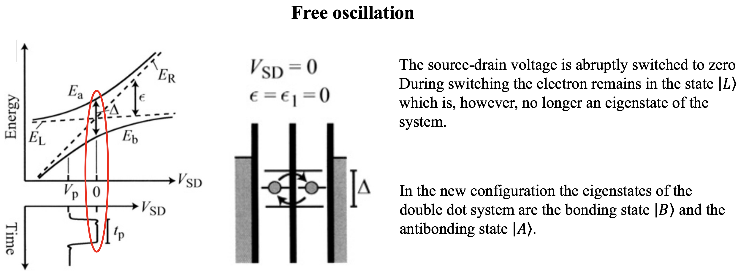
1. Bonding Orbital : This orbital is a quantum state where the wave functions of two electrons (or electron states) from neighboring quantum dots add constructively. It’s analogous to the bonding orbital in a molecule, where two atomic orbitals overlap and combine to increase the probability of finding electrons in the region between the two nuclei (or quantum dots in this case). This results in a lower energy state; the electrons are more likely to be found between the dots, which lowers the system’s potential energy. The energy associated with this orbital is lower than the original energy levels of the isolated dots, hence the energy , where the negative sign indicates a lower energy than the individual dot levels.

2. Antibonding Orbital ​: Conversely, the antibonding orbital is a quantum state where the wave functions of the electrons from the two dots combine destructively, meaning there is less probability of finding the electrons in between the dots. In molecular terms, this would correspond to a node, or a region of zero probability, between the nuclei. For quantum dots, this means that the electron wave functions do not overlap favorably, leading to a higher energy state because the electrons prefer to remain more localized to their respective dots. The antibonding orbital has a higher energy , reflecting this reduced stability and the increased energy due to the unfavorable overlap.

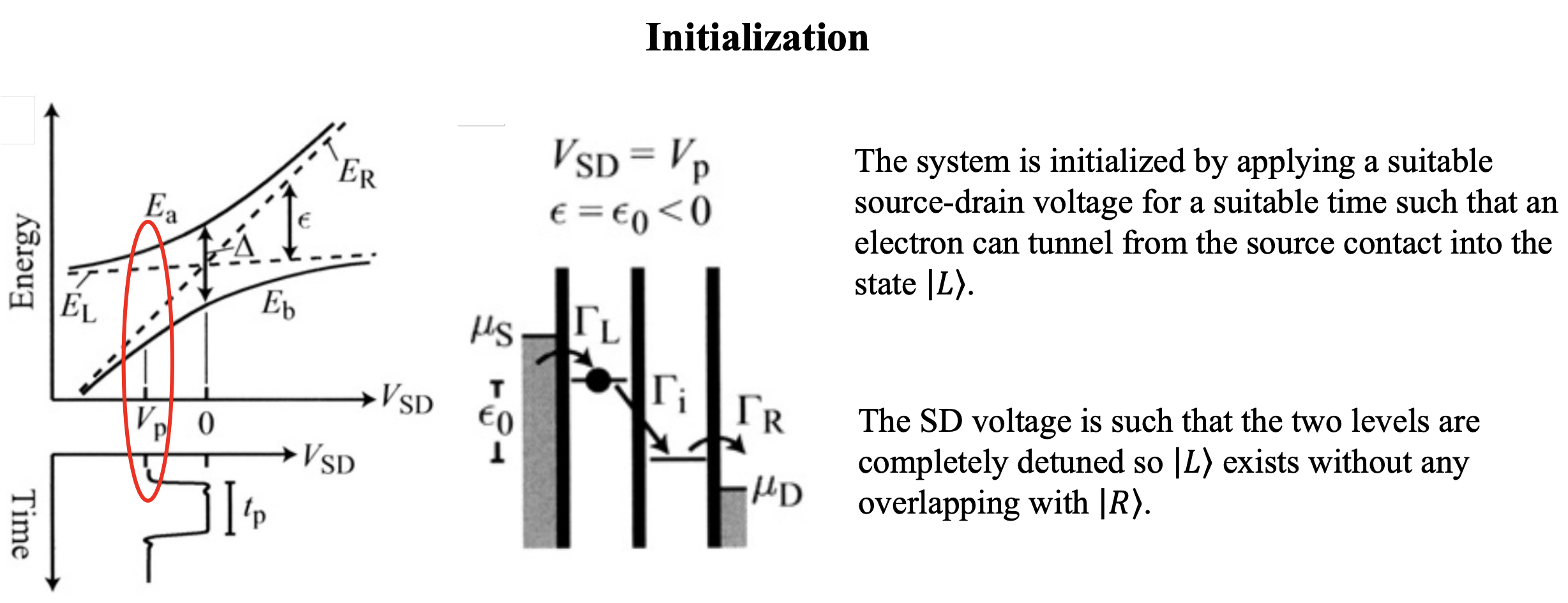
Detuning

Detuning () refers to the energy difference between the levels of two coupled quantum dots when their energy levels are not aligned.

For two coupled quantum dots, detuning is typically controlled by adjusting the gate voltages applied to the dots. These voltages shift the potential energy landscape of the electrons in the dots, thereby changing their energy levels. When the levels are aligned, electrons can tunnel freely between the dots.

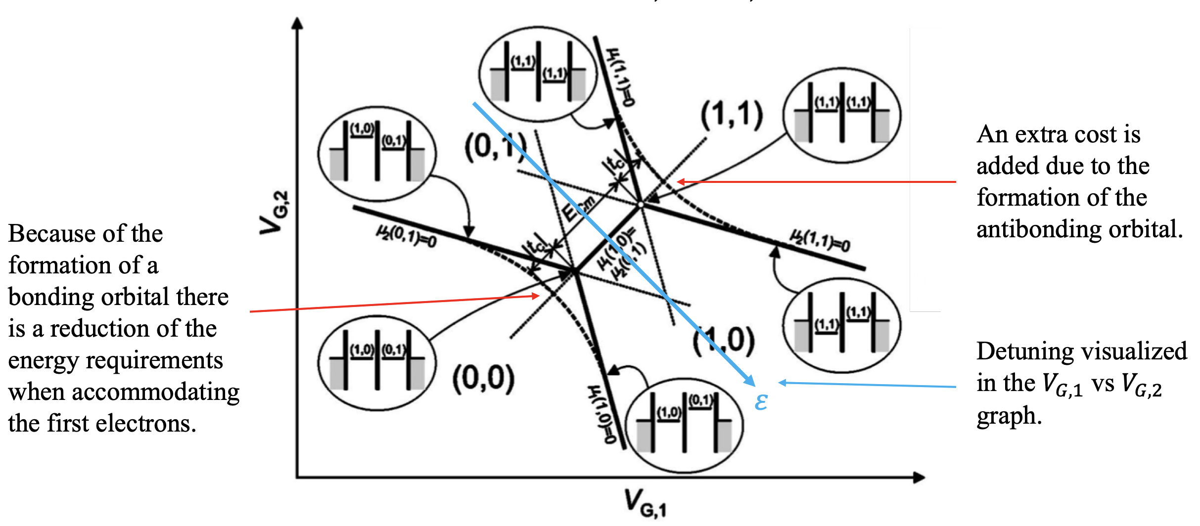
Bonding Orbital Formation: When the first electrons enter the quantum dots, they occupy the bonding orbital, a lower energy state resulting from the constructive interference of the wave functions from both dots. This means it takes less energy to add an electron because they’re effectively sharing the space between the two dots, which is energetically favorable. This is shown as a reduction of energy requirements in the diagram.

Antibonding Orbital: are shown as an extra cost in the diagram.

Detuning: This is represented by the diagonal lines in the diagram and indicates the energy difference between the levels of the two dots. When the dots are detuned, one dot’s energy level is higher or lower than the other’s. By adjusting the gate voltages, one can control the detuning and thus control the electron tunneling between the dots.

Qubit

We can use a double quantum dot structure, for example, based on a heterostructure with a two-dimensional electron gas, to create a singlequbit. Depending on the voltage we apply, the dots states are either split (large detuning) or hybridized to form bonding and antibonding orbitals (small detuning).

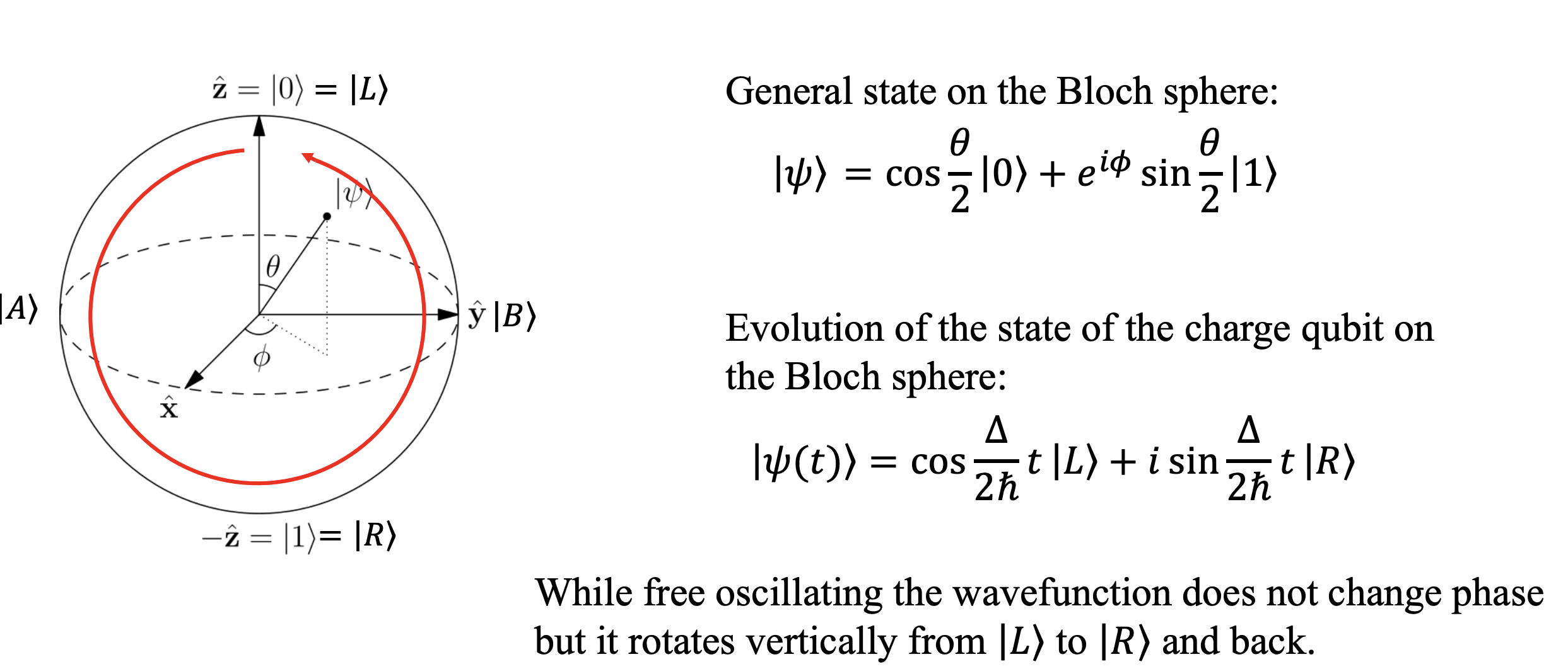
The two basis states of the qubit are taken to be the two charge states and corresponding to the electron in the left and in right dot respectively.

The bonding and antibonding states are superimpositions of the left and right states: