Entropy

Thermodynamic entropy

Formulas and definitions

• Thermodynamic parameters: measurable macroscopic quantities associated with the system (pressure, volume, temperature, etc).
• Thermodynamic state: is specified by a set of values of all the thermodynamic parameters necessary to describe the system.
• Thermodynamic equilibrium: condition when the thermodynamic state does not change in time.
• Equation of state: is a function of the thermodynamic parameters for a system in equilibrium and defines a surface .
• P-V diagram: projection of the surface of the equation of state onto the P-V plane
• Work:
• Heat: where is the heat capacity.

I law of thermodynamics

Considering an arbitrary thermodynamic transformation with the heat absorbed by the system and the work done by the system, the difference in internal energy will be given by:

which can be written in differential form as

II law of thermodynamics

The second law of thermodynamics can be expressed in two equivalent forms:

• Kelvin statement: There exists no thermodynamic transformation whose sole effect is to extract a quantity of heat from a given heat reservoir and to convert it entirely into work.
• Clausius statement: There exists no thermodynamic transformation whose sole effect is to extract a quantity of heat from a colder reservoir and to deliver it to a hotter reservoir.

Carnot engine

todo

Entropy definition

The entropy between two states (state with ) and a generic state is given by:

We are usually interested in the difference in entropy of two states, which is defined as

where the path of integration is any reversible path joining to .

The in holds for the case of reversible transformations.

Shannon entropy

This part is heavily based on the Shannon's masterpiece " A mathematical theory of communication"

We can start the analysis of the concept of entropy in the Information field by studying a discrete information source that generates a message, symbol by symbol.

A physical system, or a mathematical model of a system which produces such a sequence of symbols governed by a set of probabilities, is known as a stochastic (random) process. Examples of these systems can be a natural language, a source of information, etc.

We can start introducing the concepts that will be useful later in a simple case where we have only five letters

which each have probability of being chosen (this is called letter frequency). Let’s suppose for now that the probabilities are all equal:

We will also restrict our analysis to the case of independent choices (the probabilities of a letter is not influenced by the previous letters).

Forming a message with these rules leads to something similar to

We can slightly increase the complexity analysing a case where the probabilities (letter frequencies) are not the same. For example

A possible message in this case could be

To further complicate the structure of our system we can introduce the concept of transition probability , which indicate the probability that letter is followed by letter . This is the same as specifying the digram probability , which indicates the probability to obtain the digram .

The following properties hold for the probabilities we just saw:

We could theoretically add probabilities for trigrams and so on.

The more constraints we add, the more we approach a real language (see the paper for more examples).

At this point we would like to find a way to measure “how much information is produced”. Such measure, let’s call it , should have the following properties:

1. Should be continuous in the .
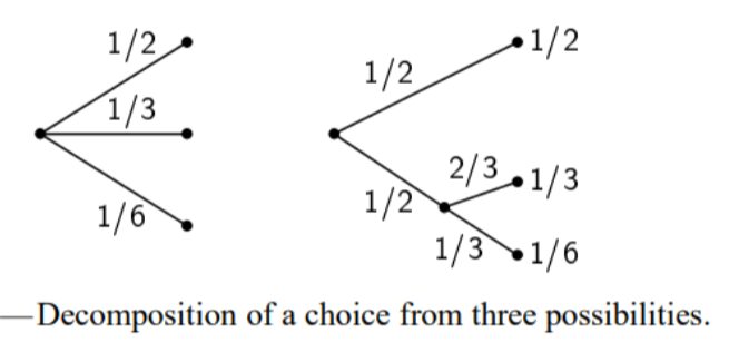
2. If all the are equal, it should be a monotonic increasing function of . This means that with equally likely events we will have more uncertainty as we increase the number of events.
3. If a choice is broken down into two successive choices, the original should be the weighted sum of the individual values of . The meaning of this statement is explained in the image below.

Theorem (Definition of Shannon entropy)

The only that satisfies the three above assumptions is of the form

where is a positive constant which is usually omitted.

Demonstration

todo

Example, binary entropy

See Nielsen Chuang, 11.2.1

In the simple case of two possibilities with probabilities and , the entropy would be

From the plot of below we can see that when the output is know (blue dots), the entropy is zero, which is to say that we have no surprise in the outcome. On the other hand, when , the entropy is equal to , which means that we don’t know what to expect.

Properties

From the example above we already noticed some interesting properties of the quantity , which are also valid in general:

1. if and only if all the except one of them, which has value .
2. For a given , has a maximum equal to when all the are equal.
3. Suppose there are two events, and , with possibilities for the first and for the second. Let be probability of the join occurrence of for the first and for the second. The entropy of the join event is:

while

It can be shown that

where the equality holds if the events are independent ().

4. Any change toward equalization of the probabilities increases . This can be easily derived from property 2.
5. If we have two events and like in property 3, not necessarily independent. For any particular value that can assume, there is a conditional probability that has the value :

Conditional entropy

We can also define the conditional entropy of , as the average of the entropy of for each value of , weighted according to the probability of getting that particular :

This quantity measures how uncertain we are of on average when we know . Substituting the value of we obtain the following relation:

Entropy measurement units

The choice of the logarithmic base corresponds to the choice of a measurement unit. The most common ones are the following:

• : bits
• : nats
• : dits or hartleys
• : bytes

Relative entropy

Given two probability distributions and , the relative entropy between the two is defined as

even though the meaning of this quantity is not obvious, we can prove that it is a good measure of distance between two probability distributions because it is non negative and it is equal to zero if and only if the two probability distributions are identical (for a proof see Nielsen Chuang, Theorem 11.1)