Circuit QED

From atomic physics to quantum optics

The idea of superconducting circuit is to “mimic” the behavior of real atoms. The great advantage of superconducting circuits is that they can be more easily tuned. As mentioned in the lecture on Superconductive qubits, the energy levels of the atoms are discrete.

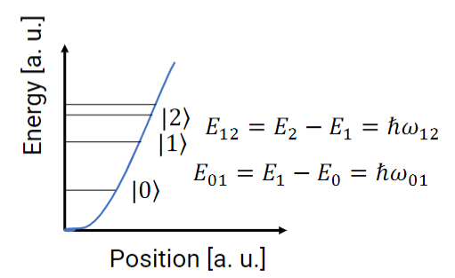
Furthermore, the quantum state of an atom can be influenced by an electromagnetic radiation, giving rise to stimulated emission and absorption. This gives some degree of freedom in controlling its state.

We will be interested in doing the same with SC circuits. But before diving into how a SC circuit can be controlled trough EM radiation, is useful to review very briefly what happens in the case of natural atoms.

In first approximation, the coupling between an atom and an electromagnetic wave is described by the interaction of the electric field with the electric dipole of the atom :

Where is a factor that describes the strength of the coupling.

To excite a transition between the state and , is possible to use an electromagnetic wave with a frequency that matches the energy difference between this two levels: . For instance the electric field can be chosen as:

Where is the amplitude of the electric field.

To increase the strength of the field, and therefore the strength of the coupling , is possible to exploit a Fabry Perot cavity.

We will not describe in detail this apparatus, we will just limit ourself in describing some of the main important facts.

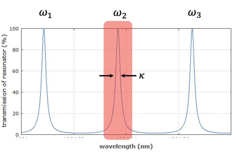
A Fabry Perot cavity (FPC) is a cavity created between two semi-reflective mirrors. A light beam can be transmitted across a FPC only if ==the frequency is “close” to a multiple of the resonant frequency of the cavity ==, that depends on its geometry.

The transmitted intensity across the FPC follows a behavieour similar to this: 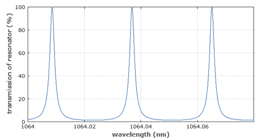Where the peaks are centered in correspondence of the resonant frequencies (or wavelengths). Under the resonant condition, stationary wave are formed inside of the cavity, giving rise to an electric field that is related to the volume of the cavity by:

Therefore the field is stronger the smaller is the cavity.

From cavity to QED

Warning

• In this section many subsequent approximation will be used. To help the reader, we have underlined with bold characters when a new approximation is introduced.
• In this notes many hamiltonians differs from the one in the professors’s slides. The professor often divided the hamiltonians by , in order to have less constants in the equations. We made the choice of maintaining the constant, in order tho have hamiltonians that are expressed as energies (and not frequencies).

To operate qubits it is possible to realize a circuit that works similarly to a FPC. A possible realization is shown is the following figure:

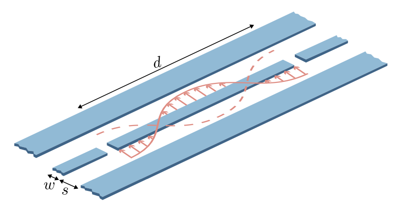
The circuit to realize the planar waveguide is obtained depositing three conductive stripes. This system works similarly to a coaxial cable: the stipe in the middle is the conductive part, that is insulated from the two external stripes, that are grounded. The FPC is created in the central conductor using the two “cuts” that are visible in the figure. This creates a stripe of length , that behaves as a resonator. In this case, the resonance condition occurs when the wavelength of the electromagnetic wave propagating trough the waveguide is a multiple of the length of the resonator.

This configuration creates a tightly confined electric field in proximity of the resonator, that can be capacitively coupled with a qubit (transmont qubit) as shown in the figure:

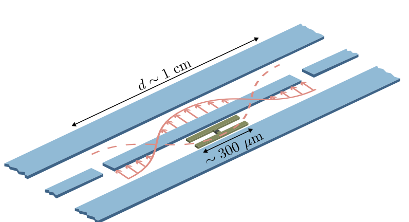
The confinement of the electric field gives rise to a measurable Zero Point Electric field (ZPE), of the order of . This is a purely quantum effect, that causes the presence of a non-zero electric field even in absence of photons (this fluctuation in the electric field value is mainly due to the Heisenberg uncertainty principle).

In general the resonator has many resonant frequencies. Even so, when the circuit is operated at a frequency that is colse to a particular resonating frequency , is possible to neglect all the other resonating modes.

Under this approximation, called one mode approximation, the resonator can be treated as an armonic oscillator (LC circuit) with a frequency ( in the image below).

 is the width of the peak at half-amplitude:

where is the quality factor, same parameter the we encounter in standard filters.

Taking into account this approximation the system can be schematized using the following lumped element model:

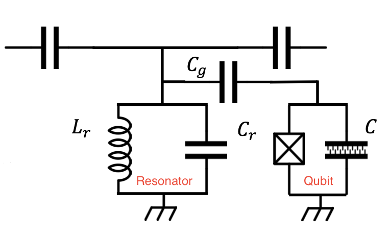
Where is a capacitative term that describes the coupling between the Qubit and the resonator.

To understand how the system behaves we need to write a suitable Hamiltonian. If the Resonator and the Qubit were not interacting, the hamiltonian would be just the sum of the two single Hamiltonians:

Where in writing the final form of , the same approximation as in Superconductive qubits has been used. Since the two are capacitatively coupled, to describe the system is essential to add a term that takes this interaction into account: .

The factor , as in the case of natural atoms, is a quantity that describes the strength of the interaction. The interaction term is proportional to the product of the operators , this brings us a step closer to understand the physical meaning of this term, but not sufficiently close to really grasp its deep essence. Perhaps it is not even important, since it is not explained even in the papers.

Since the qubit is operated in a regime where only the two least energetic levels are accessible, the more general operators and can be replaced with the operators and respectively, that act on a two level system.

We recall that the definitions of and :

This approximation can be regarded as two levels system approximation. To further simplify the model is possible to neglect the high frequency terms, applying the rotating waves approximation, already introduced in the chapter about Superconductive qubits.

We summarize here the main steps and approximations that lead to the so called Jaynes-Cummings Hamiltonian (boxed):

with:

• 1. Single mode approximation, approximated interaction term and approximated
• 2. Two levels approximation
• 3. Rotating waves approximation

In the interaction term, describes the destruction of an excitation of the qubit with the creation on a photon, while describes the creation on an excitation for the annihilation of a photon. Therefore, now the interaction term has the following interpretation: the qubit can:

• Go from to absorbing one photon.
• Go from to emitting one photon.

The Jaynes-Cummings Hamiltonian can be solved exactly and used to describe many situations in which an atom, artificial or natural, can be considered a two-level system in interaction with an electromagnetic field. In our case, the interaction described by this hamiltonian will be useful to control the state of the qubit.

Approximations to further simplify the model can be done in the dispersive regime, that occurs if the resonating frequency of the qubit and the bare resonating frequency are sufficiently far apart. This can be expressed more formally asking that the contribute to the energy of the coupling needs to be smaller than the energy difference between the resonant energies of the qubit and the resonator:

Where is called “detuning”.

Under this condition it is possible to treat the interaction term with perturbation theory, leading to the following result:

Where is called “Dispersive interaction term” and is the pauli z-matrix that acts on the qubit state. The important thing to notice is that now the actual resonator frequency depends on the state of the qubit, and is equal to:

• if the state of the qubit is
• if the state of the qubit is

This can be exploited for the readout of the qubit state.

Control and readout of one qubit

The state readout is performed in dispersive regime, using a frequency 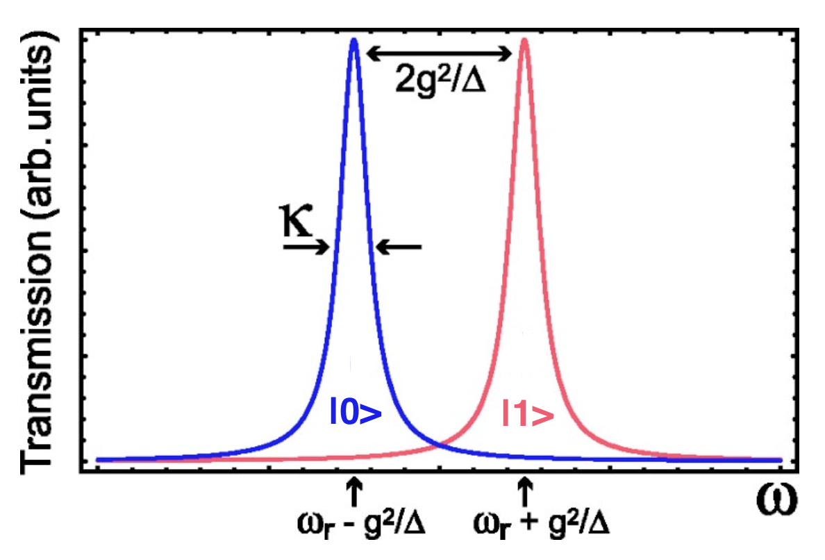close to the resonance frequency of the bare resonator . Under this condition the transmitted spectra depend on the state of the qubit as shown in this picture: So, by observing what is the resonance frequency one can perform a measure on the qubit state. If the resonance frequency is shifted up (down), means that the qubit collapsed in the state ().

Is important to stress that operating in the dispersive regime allows to perform a non destructive measurement on the qubit. This means that the perturbation induced by the readout process makes the qubit collapse without affecting its state before the measurement.

This is made possible by the fact that the driving frequency is “close” to the resonant frequency, and is “far” from the resonant frequency of the qubit.

Instead the state control can be performed using a frequency that matches the frequency between the two states of the qubit . Since in this case the driving frequency is different from the resonance frequency, the incoming signal will be almost completely reflected. Even so, some photons with frequency can still enter in the cavity, and interact with the qubit affecting Jaynes-Cummings Hamiltonian, thus affecting its state.

Multiple qubits control and readout

With the same circuit, is possible to put multiple qubit near the resonator in order to have a many-qubit system. An actual possible implementation is schematized in this figure: Each of the qubit can be designed in order to have its own operating frequency . This makes possible:

• individual state control: using a driving frequency one can control the state of the i-th qubit.
• global readout: using a driving frequency , one will obtain a transmission spectrum with a pattern that will be affected by the state of each qubit.

Xmon qubit

The papers from which this lecture is based on, used a Transmon realized with an interdigital capacitor:

Still, the presented derivation holds for any implementation of the trasmon qubit. All the theory remains untouched, from the lumped element circuit to the derivation of the hamiltonian.

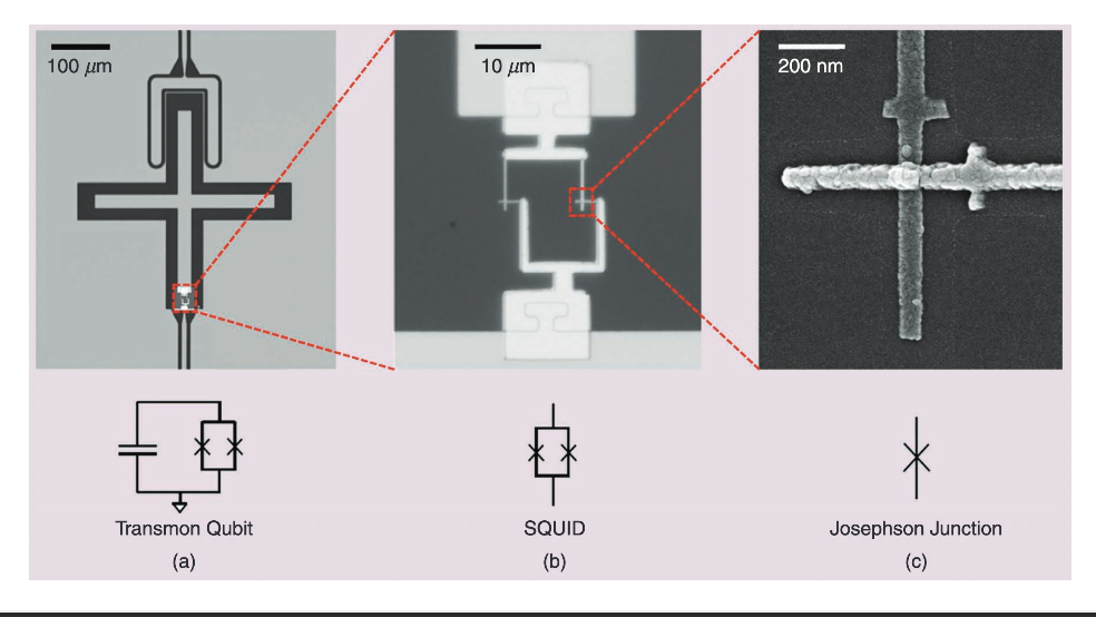
A particular, very convenient, implementation is the xmon qubit. This name comes after its cross-shaped geometry.

This configuration brings several advantages:

• Interconnectivity: “easy” to couple to other qubits, to measurement instruments or to control lines.
• Tunability: can be tuned replacing the Josephson junction with a squid

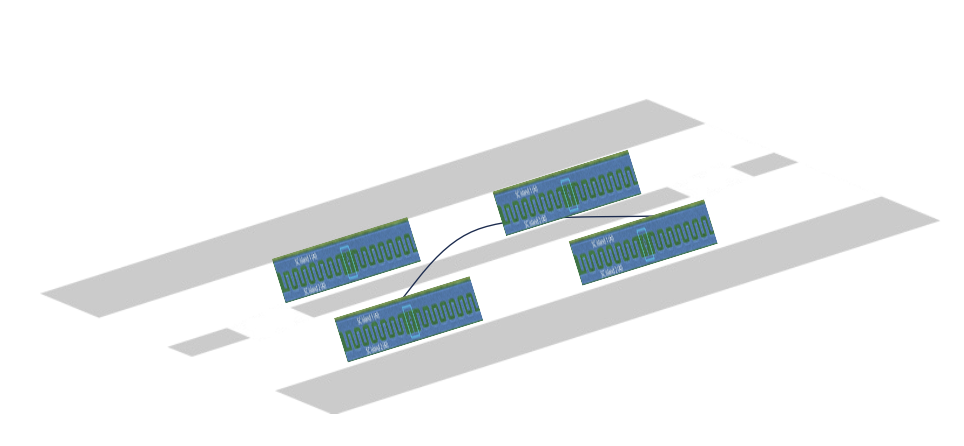
Here is reported an array of five connected Xmon qubits, coupled with transmission and control line:

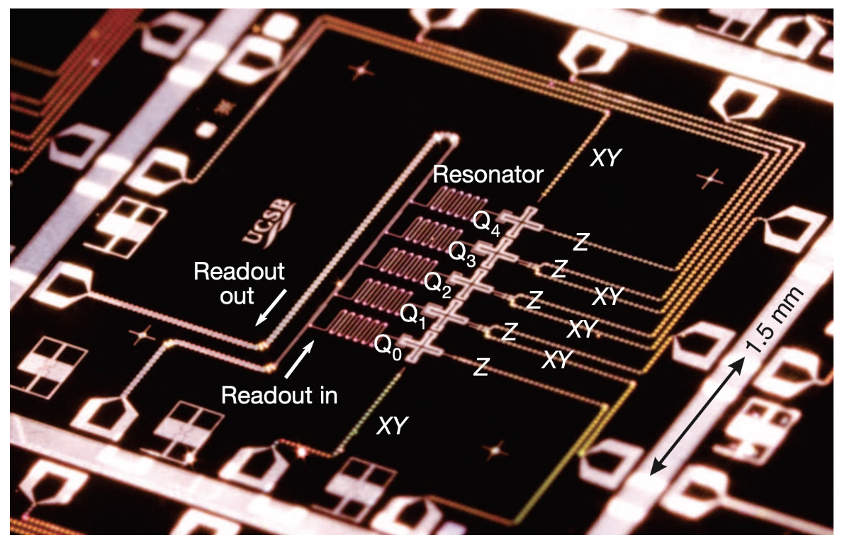We can notice the cross-shaped transmon qubits that are coupled by simply placing them one close to the other; for every qubit, we have CONTROL LINES used for x-y control, and z-line which is used to tune the frequency of the qubit (NOT for z-rotation!).

Sending specific pulses to the z line allows to tune the frequency of the qubit during the operation.
Moreover, instead of a cavity the resonator is done using a planar waveguide, which is much more practical. In order to read, we have an input port (READOUT IN) where we transmit a signal, which is in turn affected by the state of every qubit and then comes to the output (READOUT OUT), where the information can be read and processed, so to understand which was the state of the qubit.

We now need to understand how we can control x and y, i.e. what is the signal to send to perform the rotation (combining them, we can also obtain a z rotation).

Further readings: https://doi.org/10.1103/RevModPhys.93.025005 https://doi.org/10.1103/PhysRevA.69.062320